Mitigating Bias in Machine Learning
Part I Introduction
Welcome to Mitigating Bias in Machine Learning. If you’ve made it here chances are you’ve worked with models and have some awareness of the problem of biased machine learning algorithms. You might be a student with a foundational course in machine learning under your belt, or a Data Scientist or Machine Learning Engineer, concerned about the impact your models might have on the world.
In this book we are going to learn and analyse a whole host of techniques for measuring and mitigating bias in machine learning models. We’re going to compare them, in order to understand their strengths and weaknesses. Mathematics is an important part of modelling, and we won’t shy away from it. Where possible, we will aim to take a mathematically rigorous approach to answering questions.
Mathematics, just like code, can contain bugs. In this book, each has been used to verify the other. The analysis in this book, was completed using Python. The Jupyter Notebooks are available on GitHub, for those who would like to see/use them. That said, this book is intended to be self contained, and does not contain code. We will focus on the concepts, rather than the implementation.
Mitigating Bias in Machine Learning is ultimately about fairness. The goal of this book is to understand how we, as practising model developers, might build fairer predictive systems and avoid causing harm (sometimes that might mean not building something at all). There are many facets to solving a problem like this, not all of them involve equations and code. The first two chapters (part I) are dedicated to discussing these.
In a sense, over the course of the book, we will zoom in on the problem, or rather narrow our perspective. In chapter 1, we’ll discuss philosophical, political, legal, technical and social perspectives. In chapter two we take a more practical view on the problem of ethical development (how to build and organise the development of models, with a view to reducing ethical risk).
In part II we will talk about how we quantify different notions of fairness.
In part III, we will look at methods for mitigating bias through model interventions and analyse their impact.
Let’s get started.
1 Context
This chapter at a glance
Problems with machine learning in sociopolitical domains
Contrasting socio-political theories of fairness in decision systems
The history, application and interpretation of anti-discrimination law
Association paradoxes and the difficulty in identifying bias
The different types of harm caused by biased systems
The goal of this chapter is to shed light on the problem of bias in machine learning, from a variety of different perspectives. The word bias can mean many things but in this book, we use it interchangeably with the term unfairness. We’ll talk about why later.
Perhaps the biggest challenge in developing sociotechnical systems is that it inevitably involve questions which are social, philosophical, political, and legal in nature; questions to which there is often no definitive answer but rather competing viewpoints and trade-offs to be made. As we’ll see, this does not change when we attempt to quantify the problem. There are many multiple definitions of fairness that have been proven to be impossible to satisfy simultaneously. The problem of bias in sociotechnical systems is very much an interdisciplinary one and, in this chapter, we discuss them as such. We will make connections between concepts and language from the various subjects over the course of this book.
In this chapter we shall discuss some philosophical theories of fairness in sociopolitical systems and consider how they might relate to model training and fairness criteria. We’ll take a legal perspective, looking at anti-discrimination laws in the US as an example. We’ll discuss some of the history behind and practical application of them; and the tensions that exist in their interpretation. Data can be misleading; correlation does not imply causation which is why domain knowledge in building sociotechnical systems is imperative. We will discuss the technical difficulty in identifying bias in static data through illustrative examples of Simpson’s paradox. Finally, we’ll discuss why it’s important to consider the fairness of automated systems. We’ll finish the chapter by discussing some of the different types of harm caused by biased machine learning systems, not just allocative but representational harms which are currently less well defined and potentially valuable research areas.
Let’s start by describing the types of problems we are interested in.
1.1 Bias in Machine Learning
Machine learning can be described as the study of computer algorithms that improve with (or learn) experience. It can be broadly subdivided into the fields of supervised, unsupervised and reinforcement learning.
Supervised learning
For supervised learning problems, the experience come in the form of labelled training data. Given a set of features \(X\) and labels (or targets) \(Y\), we want to learn a function or mapping \(f\), such that \(Y = f(X)\), where \(f\) generalizes to previously unseen data.
Unsupervised learning
For unsupervised learning problems there are no labels \(Y\), only features \(X\). Instead we are interested in looking for patterns and structure in the data. For example, we might want to subdivide the data into clusters of points with similar (previously unknown) characteristics or we might want to reduce the dimensionality of the data (to be able to visualize it or simply to make a supervised learning algorithm more efficient). In other words, we are looking for a new feature \(Y\) and the mapping \(f\) from \(X\) to \(Y\).
Reinforcement learning
Reinforcement learning is concerned with the problem of optimally navigating a state space to reach a goal state. The problem is framed as an agent that takes actions, which result in rewards (or penalties). The task is then to maximize the cumulative reward. As with unsupervised learning, the agent is not given a set of examples of optimal actions in various states, but rather must learn them through trial and error. A key aspect of reinforcement learning is the existence of a trade-off between exploration (searching unexplored territory in the hope of finding a better choice) and exploitation (exploiting what has been learned so far).
In this we will focus on the first two categories (essentially algorithms that capture and or exploit patterns in data), primarily because these are the fields in which problems related to bias in machine learning are most pertinent (automation and prediction). As one would expect then, these are also the areas in which many of the technical developments in measuring and mitigating bias have been concentrated.
The idea that the kinds of technologies described above are learning is an interesting one. The analogy is clear, learning by example is certainly a way to learn. In less modern disciplines one might simply think of training a model as; solving an equation, interpolating data, or optimising model parameters. So where does the terminology come from? The term machine learning was coined by Arthur Samuel in the 1950’s when, at IBM, he developed an algorithm capable of playing draughts (checkers). By the mid 70’s his algorithm was competitive at amateur level. Though it was not called reinforcement learning at the time, the algorithm was one of the earliest implementations of such ideas. Samuel used the term rote learning to describe a memorisation technique he implemented where the machine remembered all the states it had visited and the corresponding reward function, in order to extend the search tree.
1.1.1 What is a Model?
Underlying every machine learning algorithm is a model (often several of them) and these have been around for millennia. Based on the discovery of palaeolithic tally sticks (animal bones carved with notches) it’s believed that humans have kept numerical records for over 40,000 years. The earliest mathematical models (from around 4,000 BC) were geometric and used to advance the fields of astronomy and architecture. By 2,000 BC, mathematical models were being used in an algorithmic manner to solve specific problems by at least three civilizations (Babylon, Egypt and India).
A model is a simplified representation of some real world phenomena. It is an expression of the relationship between things; a function or mapping which, given a set of input variables (features), returns a decision or prediction (target). A model can be determined with the help of data, but it need not be. It can simply express an opinion as to how things should be related.
If we have a model which represents a theoretical understanding of the world (under a series of simplifying assumptions) we can test it by measuring and comparing the results to reality. Based on the results we can assess how accurate our understanding of the world was and update our model accordingly. In this way, making simplifying assumptions can be a means to iteratively improve our understanding of the world. Models play an incredibly important role in the pursuit of knowledge. They have provided a mechanism to understand the world around us, and explain why things behave as they do; to prove that the earth could not be flat, explain why the stars move and shift in brightness as they do or, (somewhat) more recently in the case of my PhD, explain why supersonic flows behave uncharacteristically, when a shock wave encounters a vortex.
As the use of models has been adopted by industry, increasingly their purpose has been geared towards prediction and automation, as a way to monetize that knowledge. But the pursuit of profit inevitably creates conflicts of interests. If your goal is to learn more, finding out where your theory is wrong and fixing it is the goal. In business, less so. I recall a joke I heard at school describing how one could tell which field of science an experiment belonged to. If it changes colour, it’s biology; if it explodes, it’s chemistry and if it doesn’t work, it’s physics. Models of real world phenomena fail. They are, by their very nature, a reductive representation of an infinitely more complex real world system. Obtaining adequately rich and relevant data is a major limitation of machine learning models and yet, they are increasingly being applied to problems, where that kind of data simply doesn’t exist.
1.1.2 Sociotechnical systems
We use the term sociotechnical systems to describe systems that involve algorithms that manage people. They make efficient decisions for and about us, determine what we see, direct us and more. But managing large numbers of people inevitably exerts a level of authority and control. An extreme example is the adoption of just-in-time scheduling algorithms by large retailers in the US to manage staffing needs. To predict footfall, the algorithms take into account everything from weather forecasts to sporting events. The cost of this efficiency is passed onto employees. The number of hours allocated are optimised to fall short of qualifying for costly health insurance. Employees are subjected to haphazard schedules that prevent them from being able to prioritise anything other than work; eliminating the possibility of any opportunity that might enable them to advance beyond the low-wage work pool.
Progress in the field of deep learning combined with increased availability and decreased cost of computational resources has led to an explosion in data and model use. Automation seemingly offers a path to making our lives easier, improving the efficiency and efficacy of the many industries we transact with day to day; but there are growing and legitimate concerns over how the benefit (and cost) of these efficiencies are distributed. Machine learning is already being used to automate decisions in just about every aspect of modern life; deciding which adverts to show to whom, deciding which transactions might be fraud when we shop, deciding who is able to access to financial services such as loans and credit cards, determining our treatment when sick, filtering candidates for education and employment opportunities, in determining which neighbourhoods to police and even in the criminal justice system to decide what level bail should be set at, or the length of a given sentence. At almost every major life event, going to university, getting a job, buying a house, getting sick, decisions are being made by machines.
1.1.3 What Kind of Bias?
The word bias is rather overloaded; it has numerous different interpretations even within the same discipline. Let’s talk about the kinds of biases that are relevant here. The word bias is used to describe systematic errors in variable estimation (predictions) from data. If the goal is to create systems that work similarly well for all types of people, we certainly want to avoid these. In a social context, bias is spoken of as prejudice or discrimination in a given context, based on characteristics that we as a society deem to be unacceptable or unfair (for example hiring practices that systematically disadvantage women). Mitigating bias though is not just about avoiding discriminating, it can also manifest when a system fails to adequately discriminate based on characteristics that are relevant to the problem (for example systematically higher rates of error in visual recognition systems for darker skinned individuals). Systemic bias and discrimination are observed in data in numerous ways; historical decisions of course are susceptible, but more importantly perhaps in the very definition of the categories, who is recognised and who is erased. Bias need not be conscious, in reality it starts at the very inception of technology, in deciding which problems are worth solving in the first place. Bias exists in how we measure the cost and benefit of new technologies. For sociotechnical systems, these are all deeply intertwined.
Ultimately, mitigating bias in our models is about fairness and in this book we shall use the terms interchangeably. Machine learning models are capable of not only of proliferating existing societal biases, but amplifying them, and are easily deployed at scale. But how do we even define fairness? And from whose perspective do we mean fair? The law can provide some context here. Laws, in many cases, define protected characteristics and domains (we’ll talk more about these later). We can potentially use these as a guide and we certainly have a responsibility to be law abiding citizens. A common approach historically has been to ignore protected characteristics. There’s a few reasons for this. One reason is the false belief that, an algorithm cannot discriminate based on features not included in the data. This assumption is is easy to disprove with a counter example. A reasonably fool-proof way to systematically discriminate by race or rather ethnicity (without explicitly using it), is to discriminate by location/residence; that is, another variable that’s strongly correlated and serves as a proxy. The legality of this practice depends on the domain. In truth, you don’t need a feature, or a proxy, to discriminate based on it, you just need enough data, to be able to predict it. If it is predictable, the information there and the algorithm is likely using it. Another reason for ignoring protected features is avoiding legal liability (we’ll talk more about this when we take a legal perspective later in the chapter).
Example: Amazon Prime same day delivery service
In 2016, analysis published by Bloomberg uncovered racial disparities in eligibility for Amazon’s same day delivery services for Prime customersTo be clear, the same day delivery was free for eligible Amazon Prime customers on sales exceeding $35. Amazon Prime members pay a fixed annual subscription fee, thus the disparity is in the level of service provided for Prime customers who are eligible verses those that are not.
[1]
[1] D. Ingold and S. Soper, “Amazon doesn’t consider the race of its customers. Should it?” Bloomberg, 2016.
. The study used census data to identify Black and White residents and plot the data points on city maps which simultaneously showed the areas that qualified for the Prime customer same day delivery. The disparities are glaring at a glance. In six major cities, New York, Boston, Atlanta, Chicago, Dallas, and Washington, DC where the service did not have broad coverage, it was mainly Black neighbourhoods that were ineligible. In the latter four cities, Black residents were about half as likely to live in neighbourhoods eligible for Amazon same-day delivery as White residents.
At the time Amazon’s process in determining which ZIP codes to serve was reportedly a cost benefit calculation that did not explicitly take race into account but for those who have seen redlining maps from the 1930’s is hard to not see the resemblance. Redlining was the (now illegal) practice of declining (or raising prices for) financial products to people based on the neighbourhood where they lived. Because neighbourhoods were racially segregated (a legacy that lives on today), public and private institutions were able to systematically exclude minority populations from the housing market and deny loans for house improvements without explicitly taking race into account. Between 1934 and 1962, the Federal Housing Administration distributed $120 billion in loans. Thanks to redlining, 98% of these went to White families.
Amazon is a private enterprise, and it is legally entitled to make decisions about where to offer services based on how profitable it is. Some might argue they have a right to be able to make those decisions. Amazon is not responsible for the injustices that created such racial disparities, but the reality is that such disparities in access to goods and services perpetuate it. If same-day delivery sounds like a luxury, it’s worth considering the context. The cities affected have a long histories of racial segregation and economic inequality resulting from systemic racism, now deemed illegal. They are neighbourhoods which to this day are underserved by brick and mortar retailers, where residents are forced to travel further and pay more for household essentials. Now we are in the midst of a pandemic, where once delivery of household goods used to be a luxury, with so many forced to quarantine, suddenly it’s become far more of a necessity. What we consider to be a necessity changes over time, it depends on where one lives, one’s circumstances and more. Finally, consider the scale of Amazon’s operations, in 2016 one third of retail e-commerce spending in the US was with Amazon (that number has since risen to almost 50%).
1.2 A Philosophical Perspective
Developing a model is not an objective scientific process, it involves making a series subjective choices. Cathy O’Neil describes them as “opinions embedded in code”. One of the most fundamental ways in which we impose our opinion on a machine learning model, is in deciding how we measure success. Let’s look at the process of training a model. We start with some parametric representation (a family of models), which you hope is sufficiently complex to be able to reflect the relationships between the variables in the data. The goal in training is to determine which model (in our chosen family) is best. The best model being the one that maximises it’s utility (from the model developers perspective).
For sociotechnical systems, our predictions don’t only impact the decision maker, they also result in a benefit (or harm) to those subjected to them. The very purpose of codifying a decision policy is often to cheaply deploy it at scale. The more people it processes, the more value there is in codifying the decision process. Another, way to look such models instead then, is as a system for distributing benefits (or harms) among a population. Given this, which model is the right one so to speak. In this section we briefly discuss some more philosophical theories relevant to these types of problems. We start with utilitarianism which is perhaps the easiest theory to draw parallels with in modelling.
1.2.1 Utilitarianism
Utilitarianism provides a framework for moral reasoning in decision making. Under this framework, the correct course of action, when faced with a dilemma, is the one that maximises the benefit for the greatest number of people. The doctrine demands that the benefits to all people are are counted equally. Variations of the theory have evolved over the years. Some differ in their notion of how benefits are understood. Others distinguish between the quality of various kinds of benefit. In a business context, one might consider it as financial benefit (and cost). Although, this in itself depends on one’s perspective. Some doctrines advocate that the impact of the action in isolation should be considered, while others ask what the impact would be if everyone in the population took the same actions.
There are some practical problems with utilitarianism as the sole guiding principle for decision making. How do we measure benefit? How do we navigate the complexities of placing a value on immeasurable and vastly different consequences? What is a life, time, money or particular emotion worth and how do we compare and aggregate them? How can one even be certain of the consequences? Longer term consequences are hard if not impossible to predict. Perhaps the most significant flaw in utilitarianism for moral reasoning, is the omission of justice as a consideration.
Utilitarian reasoning judges actions based solely on consequences, and aggregates them over a population. So, if an action that unjustly harms a minority group happens to be the one that maximises the aggregate benefit over a population, it is nevertheless the correct action to take. Under utilitarianism, theft or infidelity might be morally justified, if those it would harm are none the wiser. Or punishing an innocent person for a crime they did not commit could be justified, if it served to quell unrest among a population. For this reason it is widely accepted that utilitarianism is insufficient as a framework for decision making.
Utilitarianism is a flavour of consequentialism, a branch of ethical theory that holds that consequences are the yard stick against which we must judge the morality of our actions. In contrast deontological ethics judges the morality of actions against a set of rules that define our duties or obligations towards others. Here it is not the consequences of our actions that matter but rather intent.
The conception of utilitarianism is attributed to British philosopher Jeremy Bentham who authored the first major book on the topic An Introduction to the Principles of Morals and Legislation in 1780. In it Bentham argues that, it is the pursuit of pleasure and avoidance of pain alone that motivate individuals to act. Given this he saw utilitarianism as a principle by which to govern. Broadly speaking, the role of government, in his view, was to assign rewards or punishments to actions, in proportion to the happiness or suffering they produced among the governed. At the time, the idea that the well-being of all people should be counted equally, and that that morality of actions should be judged accordingly was revolutionary. Bentham was a progressive in his time, he advocated for women’s rights (to vote, hold office and divorce), decriminalisation of homosexual acts, prison reform and the abolition of slavery and more. He argued many of his beliefs as a simple economic calculation of how much happiness they would produce. Importantly, he didn’t claim that all people were equal, but rather only that their happiness mattered equally.
Times have changed. Over the last century, as civil rights have advanced, the weaknesses of utilitarianism in practice have been exposed time and time again. Utilitarian reasoning has increasingly been seen as hindering social progress, rather than advancing it. For example, utilitarian arguments were used by Whites in apartheid South Africa, who claimed that all South Africans were better-off under White rule, and that a mixed government would lead to social decline as it had in other African nations. Utilitarian reasoning has been used widely by capitalist nations in the form of trickle-down economics. The theory being that the benefits of tax-breaks for the wealthy drive economic growth and ‘trickle-down’ to the rest of the population. But evidence suggests that trickle-down economic policies in more recent decades have done more damage than good, increasing national debt and fuelling income inequality. Utilitarian principles have also been tested in the debate over torture, capturing a rather callous conviction, one where the ‘means justify the ends’.
Historian and author, Yuval Noah Harari has eloquently abstracted this problem. He argues that historically, decentralization of power and efficiency have aligned; so much so, that many of us cannot think of democracy as being capable of failing, to more totalitarian regimes. But in this new age, data is power. We can train enormous models, that require vast amounts of data, to process people en masse, organise and sort them. And importantly, one does not have to have a perfect system in order to have an impact because of the scale on which they can be deployed. The question Yuval poses is, might the benefits of centralised data, offer a great enough advantage, to tip the balance of efficiency, in favour of more centralised models of power?
1.2.2 Justice as Fairness
In his theory Justice As Fairness[2] [2] J. Rawls, Justice as fairness: A restatement. Cambridge, Mass.: Harvard University Press, 2001. , John Rawls takes a different approach. He describes an idealised democratic framework, based on liberal principles and explains how unified laws can be applied (in a free society made up of people with disparate world views) to create a stable sociopolitical system. One where citizens would not only freely co-operate, but further advocate. He described a political conception of justice which would:
grant all citizens a set of basic rights and liberties
give special priority to the aforementioned rights and liberties over demands to further the general good, e.g. increasing the national wealth
assure all citizens sufficient means to make use of their freedoms.
The special priority given to the basic rights and liberties in the political conception of justice contrasts with a utilitarian doctrine. Here constraints are placed on how benefits can be distributed among the population and a strategy for determining some minimum.
Principles of Justice as Fairness
Liberty principle: Each person has the same indefeasible claim to a fully adequate scheme of equal basic liberties, which is compatible with the same scheme of liberties for all;
Equality principle: Social and economic inequalities are to satisfy two conditions:
Fair equality of opportunity: The offices and positions to which they are attached are open to all, under conditions of fair equality of opportunity;
Difference (maximin) principle They must be of the greatest benefit to the least-advantaged members of society.
The principles of Justice as Fairness are ordered by priority so that fulfilment of the liberty principle takes precedence over the equality principles and fair equality of opportunity takes precedence over the difference principle.
The first principle grants basic rights and liberties to all citizens which are prioritised above all else and cannot be traded for other societal benefits. It’s worth spending a moment thinking about what those rights and liberties look like. They are the the basic needs that are important for people to be free, to have choices and the means to pursue their aspirations. Today many of what Rawls considered to be basic rights and liberties are allocated algorithmically; education, employment, housing, healthcare, consistent treatment under the law to name a few.
The second principle requires positions to be allocated meritocratically, with all similarly talented (with respect to the skills and competencies required for the position) individuals having the same chance of attaining such positions i.e. that allocation of such positions should be independent of social class or background. We will return to the concept of equality of opportunity in chapter 3 when discussing Group Fairness.
The third principle acts to prevent redistribution of social and economic currency from the rich to the poor by requiring that inequalities are of maximal benefit to the least advantaged in a society, also described as the maximin principle. In this principle, Rawls does not take the simplistic view that inequality and fairness are mutually exclusive but rather concisely articulates when the existence of inequality becomes unfair. In a sense Rawls opposes utilitarian thinking (that everyone matters equally) in prioritising the least advantaged. We shall return to maximin principle when we look at the use of inequality indices to measure algorithmic unfairness in a later chapter.
1.3 A Legal Perspective
It’s important to remember that anti-discrimination laws are the result of long-standing and systemic discrimination against oppressed people. Their existence is a product of history; subjugation, genocide, civil war, mass displacement of entire communities, racial hierarchies and segregation, supremacist policies (exclusive access to publicly funded initiatives), voter suppression and more. The law provides an important historical record of what we as a society deem fair and unfair, but without history there is no context. The law does not define the benchmark for fairness. Laws vary by jurisdiction and change over time and in particular they often do not adequately recognise or address issues related to discrimination that are known and accepted by the sciences (social, mathematical, medical,...).
In this section we’ll look at the history, practical application and interpretation of the law in the US (acknowledging the narrow scope of our discussion) Finally, we’ll take a brief look at what might be on the legislative horizon for predictive algorithms, based on more recent global developments.
1.3.1 A Brief History of Anti-discrimination Law in the US
Anti-discrimination laws in the US rest on the 14th amendment to the constitution which grants citizens equal protections of the law. Class action law suit Brown v Board (of Education of Topeka, Kansas) was a landmark case which in 1954, legally ended racial segregation in the US. Justices ruled unanimously that racial segregation of children in public schools was unconstitutional, establishing the precedent that “separate-but-equal” was, in fact, not equal at all. Though Brown v Board did not end segregation in practice, resistance to it in the south fuelled the civil rights movement. In the years that followed the NAACP (National Association for the Advancement of Coloured People) challenged segregation laws. In 1955, Rosa parks refusing to give up her seat on a bus in Montgomery (Alabama) led to sit ins and boycotts, many of them led by Martin Luther King Jr. The resulting Civil rights act of 1964 eventually brought an end to “Jim Crow” laws which barred Blacks from sharing buses, schools and other public facilities with Whites.
After the violent attack by Alabama state troopers on participants of a peaceful march from Selma to Montgomery was televised, The Voting Rights Act of 1965 was passed. It overcame many barriers (including literacy tests), at state and local level, used to prevent Black people from voting. Before this incidents of voting officials asking Black voters to “recite the entire Constitution or explain the most complex provisions of state laws”[3] [3] P. L. B. Johnson, “Speech to a joint session of congress on march 15, 1965,” Public Papers of the Presidents of the United States, vol. I, entry 107, pp. 281–287, 1965. in the south were common place.
In the years following the second world war, there were many attempts to pass an Equal Pay Act. Initial efforts were led by unions who feared men’s salaries would be undercut by women who were paid less for doing their jobs during the war. By 1960, women made up 37% of the work force but earned on average 59 cents for each dollar earned by men. The Equal Pay Act was eventually passed in 1963 in a bill which endorsed “equal pay for equal work”. Laws for gender equality were strengthened the following year by the Civil Rights Act of 1964.
Throughout the 1800’s the American federal government displaced Native American communities to facilitate White settlement. In 1830 the Indian Removal Act was passed in order to relocate hundreds of thousands of Native Americans. Over the following two decades, thousands of those forced to march hundreds of miles west on the perilous “Trail of Tears” died. By the middle on the century, the term “manifest destiny” was popularised to describe the belief that White settlement in North America was ordained by God. In 1887, the Dawes Act laid the groundwork for the seizing and redistribution of reservation lands from Native to White Americans. Between 1945 and 1968 the federal government terminated recognition of more than 100 tribal nations placing them under state jurisdiction. Once again Native Americans were relocated, this time from reservations to urban centres.
In addition to displacing people of colour, the federal government also enacted policies that reduced barriers to home ownership almost exclusively for White citizens - subsidizing the development of prosperous "White Caucasian" tenant/owner only suburbs, guaranteeing mortgages and enabling access to job opportunities by building highway systems for White commuters, often through communities of colour, simultaneously devaluing the properties in them. Even government initiatives aimed at helping veterans of World War II to obtain home loans accommodated Jim Crow laws allowing exclusion of Black people. In the wake of the Vietnam war, just days after the assassination of Martin Luther King J, the Fair Housing Act of 1968 was passed, prohibiting discrimination concerning the sale, rental and financing of housing based on race, religion, national origin or sex.
The Civil Rights Act of 1964 acted as a catalyst for many other civil rights movements, including those protecting people with disabilities. The Rehabilitation Act (1973) removed architectural, structural and transportation barriers and set up affirmative action programs. The Individuals with Disabilities Education Act (IDEA 1975) required free, appropriate public education in the least restrictive environment possible for children with disabilities. The Air Carrier Access Act (1988) which prohibited discrimination on the basis of disability in air travel and ensured equal access to air transportation services. The Fair Housing Amendments Act (1988) prohibited discrimination in housing against people with disabilities.
Title IX of the education amendments of 1972 prohibits federally funded educational institutions from discriminating against students or employees based on sex. The law ensured that schools (elementary to university level) that were recipients of federal funding (nearly all schools) provided fair and equal treatment of the sexes in all areas, including athletics. Before this few opportunities existed for female athletes. The National Collegiate Athletic Association (NCAA) offered no athletic scholarships for women and held no championships for women’s teams. Since then the number of female college athletes has grown five fold. The amendment is credited with decreasing dropout rates and increasing the numbers of women gaining college degrees.
The Equal Credit Opportunity Act was passed in 1974 when discrimination against women applying for credit in the US was rife. It was common practice for mortgage lenders to discount incomes of women that were of ’child bearing’ age or simply deny credit to them. Two years later the law was amended to prohibit lending discrimination based on race, color, religion, national origin, age, the receipt of public assistance income, or exercising one’s rights under consumer protection laws.
In 1978, congress passed the Pregnancy Discrimination Act in response to two Supreme Court cases that ruled that excluding pregnancy related disabilities from disability benefit coverage was not gender based discrimination, and did not violate the equal protection clause.
Table 1.1 shows a (far from exhaustive) summary of regulated domains with corresponding US legislation. Note that legislation in these domains extend to marketing and advertising not just the final decision.
| Domain | Legislation |
|---|---|
| Finance | Equal Credit Opportunity Act |
| Education | Civil Rights Act (1964) |
| Education Amendment (1972) | |
| IDEA (1975) | |
| Employment | Equal Pay Act(1963) |
| Civil Rights Act (1964) | |
| Housing | Fair Housing Act (1968) |
| Fair Housing Amendments Act (1988) | |
| Transport | Urban Mass Transit Act (1970) |
| Rehabilitation Act (1973) | |
| Air Carrier Access Act (1988) | |
| Public accommodationa | Civil Rights Act (1964) |
aPrevents refusal of customers.
Table 1.2 provides a list of protected characteristics under US federal law with corresponding legislation (again not exhaustive).
| Protected Characteristic | Legislation |
|---|---|
| Race | Civil Rights Act (1964) |
| Sex | Equal Pay Act (1963) |
| Civil Rights Act (1964) | |
| Pregnancy Discrimination Act (1978) | |
| Religion | Civil Rights Act (1964) |
| National Origin | Civil Rights Act (1964) |
| Citizenship | Immigration Reform & Control Act |
| Age | Age Discrimination in Employment Act (1967) |
| Familial status | Civil Rights Act (1968) |
| Disability status | Rehabilitation Act of 1973 |
| American with Disabilities Act of 1990 | |
| Veteran status | Veterans’ Readjustment Assistance Act 1974 |
| Uniformed Services Employment & Reemployment Rights Act | |
| Genetic Information | Civil Rights Act(1964) |
1.3.2 Application and Interpretation of the Law
To get an idea of how anti-discrimination laws are be applied in practice and how they might translate to algorithmic decision making, we look at Title VII of the Civil rights act of 1964 in the context of employment discrimination[4] [4] S. Barocas and A. D. Selbst, “Big data’s disparate impact,” Calif Law Rev., vol. 104, pp. 671–732, 2016. . Legal liability for discrimination against protected classes can be established as disparate treatment and/or disparate impact. Disparate treatment (also described as direct discrimination in Europe) refers to both differing treatment of individuals based on protected characteristics, and intent to discriminate. Disparate impact (or indirect discrimination in Europe) does not consider intent but addresses policies and practices that disproportionately impact protected classes.
Disparate Treatment
Disparate treatment effectively prohibits rational prejudice (backed by data showing the protected feature to be correlated) as well as denial of opportunities based on protected characteristics. For an algorithm, it effectively prevents the use of protected characteristics as inputs. It’s noteworthy that in the case of disparate treatment, the actual impact of using the protected features on the outcome is irrelevant; so even if a company could show that the target variable produced by their model had zero correlation with the protected characteristic, the company would still be liable for disparate treatment. This fact is somewhat bizarre given that not using the protected feature in the algorithm provides no guarantee that the algorithm is not biased in relation to it. Indeed an organisation could very well use their data to predict the protected characteristic.
In an effort to avoid disparate treatment liability, many organisations do not even collect data relating to protected characteristics, leaving them unable to accurately measure, let alone address, bias in their algorithms, even if they might want toIn fact, I met a data scientist at a conference, who was working for a financial institution, that said her team was trying to predict sensitive features such as race and gender in order to measure bias in their algorithms.
. In summary, disparate treatment as applied today does not resolve the problem of unconscious discrimination against disadvantaged classes through their use of machine learning algorithms. Further it acts as a deterrent to ethically minded companies that might want to measure the biases in their algorithms.
Disparate treatment
Suppose a company predicts the sensitive feature and uses this as an input to its model. Should this be considered disparate treatment?
What about the case where the employer implements an algorithm, finds out that it has a disparate impact, and uses it anyway? Doesn’t that become disparate treatment? No it doesn’t and in fact, somewhat surprisingly, deciding not to apply it upon noting the disparate impact could result in a disparate treatment claim in the opposite direction[5] [5] “Ricci v. DeStefano, 557 U.S. 557.” 2009. . We’ll return to this later. Okay, so what about disparate impact?
Disparate Impact
In order to establish a violation, it is not enough to simply show that there is a disparate impact, but it must also be shown either that there is no business justification for it, or if there is, that the employer refuses to use another, less discriminatory, means of achieving the desired result. So how much of an impact is enough to warrant a disparate impact claim? There are no rules here only guidelines. The Uniform Guidelines on Employment selection procedures from the Equal Employment Opportunity Commission (EEOC) provides a guideline that if the selection rate from one protected group is less than four fifths of that from another, it will generally be regarded as evidence of adverse impact, though it also states that the threshold would depend on the circumstances.
Assuming the disparate impact is demonstrated, the issue becomes proving business justification. The requirement for business justification has softened in favour of the employer over the years; treated as “business necessity”[6] [6] “Griggs v. Duke Power Co., 401 U.S. 424.” 1971. earlier on and later interpreted as “business justification”[7] [7] “Wards Cove Packing Co. v. Atonio, 490 U.S. 642.” 1989. . Today, it’s generally accepted that business justification lies somewhere between the extremes of “job-relatedness” and “business necessity”. As a concrete example of disparate impact and taking the extreme of job-relatedness - the EEOC along with several federal courts have determined that discrimination on the sole basis of a criminal record to be a violation under disparate impact unless the particular conviction is related to the role, because Non-White applicants are more likely to have a criminal conviction.
For a machine learning algorithm, business justification boils down to the question of job-relatedness of the target variable. If the target variable is improperly chosen, a disparate impact violation can be established. In practice however the courts will accept most plausible explanations of job-relatedness since not accepting it would set a precedent that it is determined discriminatory. Assuming the target variable to be proven job-related then, there is no requirement to validate the model’s ability to predict said trait, only a guideline which sets a low bar (a statistical significance test showing that the target variable correlates with the trait) and which the court is free to ignore.
Assuming business justification is proven by the employer, the final burden then falls on the plaintiff to show that the employer refused to use a less discriminatory “alternative employment practice”. If the less discriminatory alternative would incur additional cost (as is likely) would this be considered refusing? Likely not.
While on the surface, disparate impact might seem like a solution, the current framework of a weak business justification (in terms of a plausible target variable) and the employer refusing an alternative employment practice with no requirement to validate the model offers little resolve. Clearly there is need for reform.
Anti-classification versus Anti-subordination
Just as the meaning of fairness is subjective so is the interpretation of anti-discrimination laws. At one extreme, anti-classification holds the weaker interpretation, that the law is intended to prevent classification of people based on protected characteristics. At the other extreme, anti-subordination defines the stronger stance, that anti-discrimination laws exist to prevent social hierarchies, class or caste systems based on protected features and, that it should actively work to eliminate them where they exist. An important ideological difference between the two schools of thought is in the application of positive discrimination policies. Under anti-subordination principles, one might advocate for affirmative action as a means to bridge gaps in access to employment, housing, education and other such pursuits, that are a direct result of historical systemic discrimination against particular groups. A strict interpretation of the anti-classification principle would prohibit such actions. Both anti-classification and anti-subordination ideologies have been argued and upheld in landmark cases.
In 2003, the Supreme Court held that a student admissions process that favours “under-represented minority groups” does not violate the Fourteenth Amendment[8] [8] “Grutter v. Bollinger, 539 U.S. 306.” 2003. , provided it evaluated applicants holistically at an individual level. The same year, the New Haven Fire Department administered a two part test in order to fill 15 openings. Examinations were governed in part by the City of New Haven. Under the city charter, civil service positions must be filled by one of the top three scoring individuals. 118 (White, Black and Hispanic) fire fighters took the exams. Of the resulting 19 candidates who scored highest on the tests and could the considered for the positions, none were Black. After heated public debate and under threat of legal action either way, the city threw out the test results. This action was later determined to be a disparate treatment violation. In 2009, the court ruled that disparate treatment could not be used to avoid disparate impact without sufficient evidence of liability of the latter[5]. This landmark case was the first example of conflict between the two doctrines of disparate impact and disparate treatment or anti-classification and anti-subordination.
Disparate treatment seems to align well with anti-classification principles, seeking to prevent intentional discrimination based on protected characteristics. In the case of disparate impact, things are less clear. Is it a secondary ‘line of defence’ designed to weed out well masked intentional discrimination? Or is its intention to address inequity that exists as a direct result of historical injustice? One can draw parallels here with the ‘business necessity’ versus ‘business justification’ requirements discussed earlier.
1.3.3 Future Legislation
In May 2018, the European Union (EU) brought into action the General Data Protection (GDPR) a legal framework around the protection of personal data of EU citizens. The framework is divided into binding and non-binding recitals. The regulation sets provisions for processing of data in relation to decision making, described as ‘profiling’ under recital 71[9] [9] “General Data Protection Regulation (GDPR): (EU) 2016/679 Recital 71.” 2016. . Though currently non-binding, it provides an indication of what’s to come. The recital talks specifically about having the right not to be subject to decisions based solely on automated processing. It specifically talks about credit applications, e-recruiting and any system which analyses or predicts aspects of a persons performance at work, economic situation, health, personal preferences or interests, reliability or behaviour, location or movements. The recital also talks about requirements around using “appropriate mathematical or statistical procedures” to prevent “discriminatory effects on natural persons on the basis of racial or ethnic origin, political opinion, religion or beliefs, trade union membership, genetic or health status or sexual orientation”. More recently in 2021, the EU has proposed taking a risk based approach to the question of which technologies should be regulated, dividing it into four categories. Unacceptable risk, high risk, limited risk, minimal risk[10] [10] “Europe fit for the Digital Age: Commission proposes new rules and actions for excellence and trust in Artificial Intelligence.” 2021. . While things may change as the proposed law is debated but once agreed, it’s not unlikely that it will serve as a prototype for legislation in the U.S. (and other countries around the world), as did GDPR.
In April 2019, the Algorithmic Accountability Act was proposed to the US Senate. The bill requires specified commercial entities to conduct impact assessments of automated decision systems and specifically states that assessments must include evaluations and risk assessment in relation to “accuracy, fairness, bias, discrimination, privacy, and security” not just for the model output but for the training data. The bill has cosponsors in 22 states and has been referred to the Committee on Commerce, Science, and Transportation for review. These examples are clear indications that the issues of fairness and bias in automated decision making systems are on the radar of regulators.
1.4 A Technical Perspective
The problem of distinguishing correlation from causation is an important one in identifying bias. Using illustrative examples of Simpson’s paradox, we demonstrate the danger of assuming causal relationships based on observational data.
1.4.1 Simpson’s Paradox
In 1973, University of California, Berkeley received approximately 15,000 applications for the fall quarter[11] [11] P. J. Bickel, E. A. Hammel, and J. W. O’Connell, “Sex bias in graduate admissions: Data from berkeley,” Science, vol. 187, Issue 4175, pp. 398–404, 1975. . At the time it was made up of 101 departments. 12,763 applications reached the decision stage. Of these 8442 were male and 4321 were female. The acceptance rates for the applicants were 44% and 35% respectively (see Table 1.3).
| Gender | Admitted | Rejected | Total | Acceptance Rate |
|---|---|---|---|---|
| Male | 3738 | 4704 | 8442 | 44.3% |
| Female | 1494 | 2827 | 4321 | 34.6% |
| Aggregate | 5232 | 7531 | 12763 | 41.0% |
With a whopping 10% difference in acceptance rates, it seems a likely case of discrimination against women. Indeed, a \(\chi^2\) hypothesis test for independence between the variables (gender and application acceptance) reveals that the probability of observing such a result or worse, assuming they are independent, is \(6\times10^{-26}\). A strong indication that they are not independent and therefore evidence of bias in favour of male applicants. Since admissions are determined by the individual departments, it’s worth trying to understand which departments might be responsible. We focus on the data for the six largest departments, shown in Table 1.4. Here again we see a similar pattern. There appears to be bias in favour of male applicants, and a \(\chi^2\) test shows that the probability of seeing this result under the assumption of independence is \(1\times10^{-21}\). It looks like we have quickly narrowed down our search.
| Gender | Admitted | Rejected | Total | Acceptance Rate |
|---|---|---|---|---|
| Male | 1198 | 1493 | 2691 | 44.5% |
| Female | 557 | 1278 | 1835 | 30.4% |
| Aggregate | 1755 | 2771 | 4526 | 38.8% |
Figure 1.1 shows the acceptance rates for each department by gender, in decreasing order of acceptance rates. Performing \(\chi^2\) tests for each department reveals the only department where there is strong evidence of bias is A, but the bias is in favour of female applicants. The probability of observing the data for department A, under the assumption of independence, is \(5\times10^{-5}\).
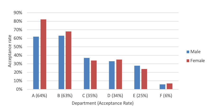
So what’s going on? Figure 1.2 shows the application distributions for male and female applicants for each of the six departments. From the plots we are able to see a pattern. Female applicants are more often applying for departments with a lower acceptance rate.
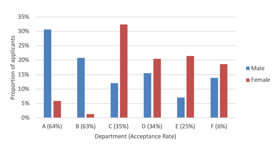
In other words a larger proportion of the women are being filtered out overall, simply because they are applying to departments that are harder to get into.
This is a classic example of Simpson’s Paradox (also known as the reversal paradox and Yule-Simpson effect). We have an observable relationship between two categorical variables (in this case gender and acceptance) which disappears or reverses, after controlling for one or more other variables (in this case department). Simpson’s Paradox is a special case of so called association paradoxes (where the variables are categorical, and the relationship changes qualitatively), but the same rules also apply to continuous variables. The marginal (unconditional) measure of association (e.g. correlation) between two variables need not be bounded by the partial (conditional) measures of association (after controlling for one or more variables). Although Edward Hugh Simpson famously wrote about the paradox in 1951, it was not discovered by him. In fact, it was reported by George Udny Yule as early as 1903. The association paradox for continuous variables was demonstrated by Karl Pearson in 1899.
Let’s discuss another quick example. A 1996 follow-up study on the effects of smoking recorded the mortality rate for the participants over a 20 year period. They found higher mortality rates among the non-smokers, 31.4% compared to 23.9% which, in itself, might imply a considerable protective affect from smoking. Clearly there’s something fishy going on. Disaggregating the data by age group showed that the mortality rates were higher for smokers in all but one of them. Looking at the age distribution of the populations of smokers and non-smokers, it’s apparent that the age distribution of the non-smoking group is more positively skewed, and so they are older on average. This concords with the rationale that non-smokers live longer - hence the difference in age distributions of the participants.
1.4.2 Causality
In both the above examples, it appears that the salient information is found in the disaggregated data (we’ll come back to this later). In both cases it is the disaggregated data that enables us to understand the true nature of the relationship between the variables of interest. As we shall see in this section, this need not be the case. To show this, we discuss two examples. In each case, the data is identical but the variables is not. The examples are those Simpson gave in his original 1951 paper[12] [12] E. Simpson, “The interpretation of interaction in contingency tables,” Journal of the Royal Statistical Society, vol. Series B, 13, pp. 238–241, 1951. .
Suppose we have three binary variables, \(A\), \(B\) and \(C\), and we are interested in understanding the relationship between \(A\) and \(B\) given a set of 52 data points. A summary of the data showing the association between variables \(A\) and \(B\) are shown in Table 1.5, first for all the data points and then stratified (separated) by the value of \(C\) (note the first table is the sum of the latter two). The first table indicates that \(A\) and \(B\) are unconditionally independent (since changing the value of one variable does not change the distribution of the other). The next two tables suggest \(A\) and \(B\) are conditionally dependent given \(C\).
| Stained? / Male? | ||||||||
|---|---|---|---|---|---|---|---|---|
| \(C=1\) | \(C=0\) | |||||||
| Black?/ Died? | Plain?/ Treated? | Black?/ Died? | Plain?/ Treated? | |||||
| \(A=1\) | \(A=0\) | \(A=1\) | \(A=0\) | \(A=1\) | \(A=0\) | |||
| \(B=1\) | 20 | 6 | \(B=1\) | 5 | 3 | 15 | 3 | |
| \(B=0\) | 20 | 6 | \(B=0\) | 8 | 4 | 12 | 2 | |
| \(\mathbb{P}(B|A)\) | 50% | 50% | \(\mathbb{P}(B|A,C)\) | 38% | 43% | 56% | 60% | |
aEach cell of the table shows the number of examples in the dataset satisfying the conditions given in the corresponding row and column headers.
Question:
Which distribution gives us the most relevant understanding of the association between \(A\) and \(B\), the marginal (i.e. unconditional) \(\mathbb{P}(A,B)\) or conditional distribution \(\mathbb{P}(A,B|C)\)? To show that causal relationships matter, we consider two different examples.
Example a) Pack of Cards (Colliding Variable)
Suppose the population is a pack of cards. It so happens that baby Milen has been messing about with the cards and made some dirty in the process. Let’s summarise our variables,
\(A\) tells us the character of the card, either plain (\(A=1\)) or royal (King, Queen, Jack; \(A=0\)).
\(B\) tells us the colour of the card, either black (\(B=1\)) or red (\(B=0\)).
\(C\) tells us if the card is dirty (\(C=1\)) or clean (\(C=0\)).
In this case, the aggregated data showing \(\mathbb{P}(A,B)\) is relevant since the cleanliness of the cards \(C\) has no bearing on the association between the character \(A\) and colour \(B\) of the cards.
Example b) Treatment Effect on Mortality Rate (Confounding Variable)
Next, suppose that the data relates to the results of medical trials for a drug on a potentially lethal illness. This time,
\(A\) tells us if the subject was treated (\(A=1\)) or not (\(A=0\)).
\(B\) tells us if the subject died (\(B=1\)) or recovered (\(B=0\)).
\(C\) tells us the gender of the subject, either male (\(C=1\)) or female (\(C=0\)).
In this case the disaggregated data shows the more relevant association, \(\mathbb{P}(A,B|C)\). From it, we can see that female patients are more likely to die than males overall; 56 and 60% versus 38 and 43%, depending on if they were treated or not. In both cases we see that treatment with the drug \(A\) reduces the mortality rate for both male and female participants, and the effect is obscured by aggregating the data over gender \(C\).
Back to Causality
The key difference between these examples is the causal relationship between the variables rather than the statistical structure of the data. In the first example with the playing cards, the variable \(C\) is a colliding variable, in the second example looking at patient mortality, it is a confounding variable. Figure 1.4 a) and b) show the causal relationships between the variables in the two cases.
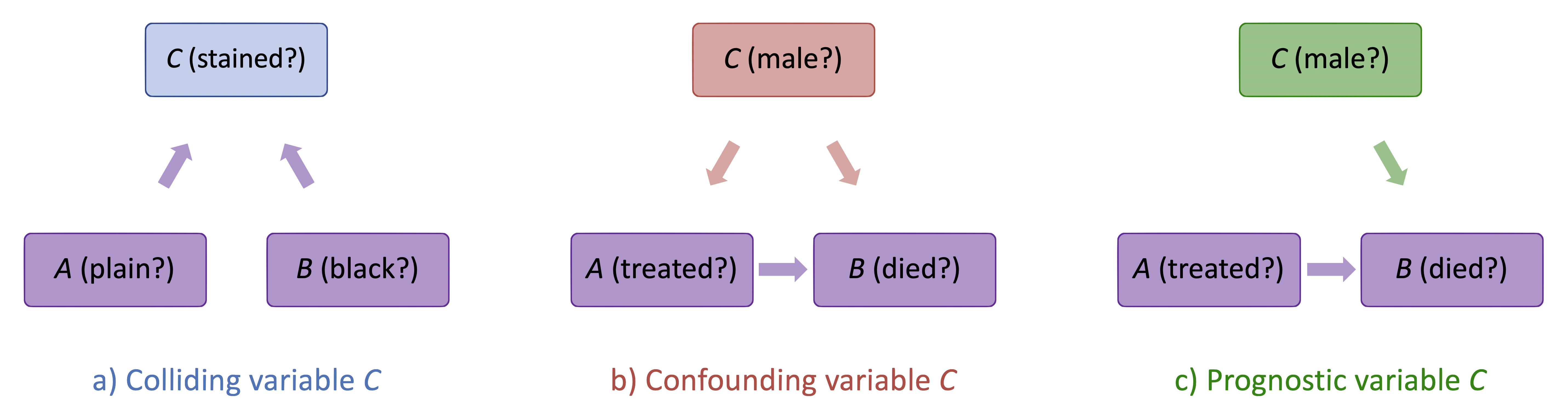
The causal diagram in Figure 1.4 a) shows the variables \(A\), \(B\) and \(C\) for the first example. The arrows exist both from card character and colour to cleanliness because apparently, baby Milen had a preference for royal cards over plain and red cards over black. Conditioning on a collider \(C\) generates an association (e.g. correlation) between \(A\) and \(B\), even if they are unconditionally independent. This common effect is often observed as selection or representation bias. Representation bias can induce correlation between variables, even where there is none. For decision systems, this can lead to feedback loops that increase the extremity of the representation bias in future data. We’ll come back to this in chapter 2, when we talk about common causes of bias.
The causal diagram in Figure 1.4 b) shows the variables \(A\), \(B\) and \(C\) for the second example. The arrows exist from \(gender\) to treatment because men were less likely to be treated, and from gender to death because men were also less likely to die. The arrow from \(A\) to \(B\) represents the effect of treatment on mortality which is observable only by conditioning on gender. Note that there are two sources of association in opposite directions between variables \(A\) and \(B\) (treatment and death); a positive association, because men were less likely to be treated; and a negative association, because male patients are less likely to die. The two effects cancel each other out when the data is aggregated.
We see through the discussion of these two examples, that statistical reasoning is not sufficient to be able to determine which of the distributions (marginal or conditional) are relevant. Note that the above conclusions in relation to colliding and confounding variables does not generalize to complex time varying problems.
Before moving on from causality, we return to the example we discussed at the very start of this section. According to our analysis of the Berkeley admissions data, we concluded that the disaggregated data contained the salient information explaining the disparity in acceptance rates for male and female applicants. The problem is, we have only shown that application rates to be one of many possible causes of the differing acceptance rates (we cannot see outside of our data). In addition, we have not proven gender discrimination, not to be the cause. What we have evidenced, is the existence of disparities in both acceptance rates and application rates across sex. One problem is that gender discrimination is not a measurable thing in itself. It’s complicated. It is made up of many components, most of which are not contained in the data. Beliefs, personal preferences, behaviours, actions, and more. A valid question we cannot answer is, why do the application rates differ by sex? How do we know that this is itself, is not a result of gender discrimination. Perhaps some departments are less welcoming of women than others or, perhaps some are just much more welcoming of men than women? So how would we know if gender discrimination is at play here? We need to ask the right questions to collect the right data.
1.4.3 Collapsibility
We have demonstrated that correlation does not imply causation in the manifestation of Simpson’s Paradox. But there is second factor that can have an impact; and that is the nature of the measure of association in question.
Example c) Treatment Effect on Mortality Rate (Prognostic Variable)
Suppose that in the study of the efficacy of the treatment (in Example 2 above), we remedy the selection bias so that male and female patients are equally likely to be treated. We remove the causal relationship between variables \(A\) and \(C\) (treatment and gender). In this case, the variable \(C\) becomes prognostic rather than confounding. See Figure 1.4 c). In this case the decision as to which distributions (marginal or conditional) are most relevant would depend only on the target population in question. In the absence of the confounding variable in our study one might reasonably expect the marginal measure of association to be bounded by the partial measures of association. Such intuition is correct only if the measure of association is collapsible (that is, it can be expressed as the weighted average of the partial measures), not otherwise. Some examples of collapsible measures of association are the risk ratio and risk difference. The odds ratio however is not collapsible. If you don’t know what these are, don’t worry, we’ll return to them in chapter 3.
1.5 What’s the Harm?
In this section we discuss the recent and broader societal concerns related to machine learning technologies.
1.5.1 The Illusion of Objectivity
One of the most concerning things about the machine learning revolution, is perception that these algorithms are somehow objective (unlike humans), and are therefore a better substitute for human judgement. This viewpoint is not just a belief of laymen but an idea that is also projected from within the machine learning community. There are often financial incentives to exaggerate the efficacy of such systems.
Automation Bias
The tendency for people to favour decisions made by automated systems despite contradictory information from non-automated sources, or automation bias, is a growing problem as we integrate more and more machines in our decision making processes especially in infrastructure - healthcare, transportation, communication, power plants and more.
It is important to be clear that in general, machine learning systems are not objective. Data is produced by a necessarily subjective set of decisions (how and who to sample, how to group events or characteristics, which features to collect). Modelling also involves making choices about how to process the data, what class of model to use and perhaps most importantly how success is determined. Finally, even if our model is calibrated to the data well, it says nothing about the distribution of errors across the population. The consistency of algorithms in decision making compared to humans (who individually make decisions on a case by case basis) is often described as a benefitOne must not confuse consistency with objectivity. For algorithms, consistency also means consistently making the same errors.
, but it’s their very consistency that makes them dangerous - capable of discriminating systematically and at scale.
Example: COMPAS
(Correctional Offender Management Profiling for Alternative Sanctions) is a “case management system for criminal justice practitioners”. The system, produces recidivism risk scores. It has been used in New York, California and Florida, but most extensively in Wisconsin since 2012, at a variety of stages in the criminal justice, from sentencing to parole. The documentation for the software describes it as an “objective statistical risk assessment tool”.
In 2013, Paul Zilly was convicted of stealing a push lawnmower and some tools in Barron County, Wisconsin. The prosecutor recommended a year in county jail and follow-up supervision that could help Zilly with “staying on the right path.” His lawyer agreed to a plea deal. But Judge James Babler upon seeing Zilly’s COMPAS risk scores overturned the plea deal that had been agreed on by the prosecution and defence, and imposed two years in state prison and three years of supervision. At an appeals hearing later that year, Babler said “Had I not had the COMPAS, I believe it would likely be that I would have given one year, six months”[13] [13] J. Angwin, J. Larson, S. Mattu, and L. Kirchner, “Machine bias,” ProPublica, 2016. . In other words the judge believed the risk scoring system to hold more insight that the prosecutor who had personally interacted with the defendant.
The Ethics of Classification
The appeal of classification is clear. It creates a sense of order and understanding. It enables us to formulate problems neatly and solve them. An email is spam or it’s not; an x-ray shows tuberculosis or it doesn’t; a treatment was effective or it wasn’t. It can make finding things more efficient in a library or online. There are lots of useful applications of classification.
We tend to think of taxonomies as objective categorisations, but often they are not. They are snapshots in time, representative of the culture and biases of the creators. The very act of creating a taxonomy, can give life by existence to some individuals, while erasing others. Classifying people inevitably has the effect of reducing them to labels; labels that can result in people being treated as members of a group, rather than individuals; labels that can linger for much longer than they should (something it’s easy to forget when creating them). The Dewey Decimal System for example, was developed in the late 1800’s and widely adopted in the 1930’s to classify books. Until 2015, it categorised homosexuality as a mental derangement.
Classification of People
From the 1930’s until the second world war, machine classification systems were used by Nazi Germany to process census data in order to identify and locate Jews, determine what property and businesses they owned, find anything of value that could be seized and finally to send them to their deaths in concentration camps. Classification systems have often been entangled with political and social struggle across the world. In Apartheid South Africa, they were been used extensively in many parts of the world to enforce social and racial hierarchies that determined everything from where people could live and work to whom they could marry. In 2019 it was estimated that some half a million Uyghurs (and other minority Muslims) are being held in internment camps in China without charge for the purposes of countering extremism and promoting social integration.
Recent papers on detecting criminality”[14] [14] X. Wu and X. Zhang, “Automated inference on criminality using face images.” 2017.Available: https://arxiv.org/abs/1611.04135 and sexuality[15] [15] Y. Wang and M. Kosinski, “Deep neural networks are more accurate than humans at detecting sexual orientation from facial images,” Journal of Personality and Social Psychology, 2018. and ethnicity[16] [16] C. Wang, Q. Zhang, W. Liu, Y. Liu, and L. Miao, “Facial feature discovery for ethnicity recognition,” Wiley Interdisciplinary Reviews: Data Mining and Knowledge Discovery, 2018. from facial images have sparked controversy in the academic community. The latter in particular looks for facial features that identify among others, Chinese Uyghurs. Physiognomy (judging character from the physical features of a persons face) and phrenology (judging a persons level of intelligence from the shape and dimensions of their cranium) have historically been used as pseudo-scientific tools of oppressors, to prove the inferiority races and justify subordination and genocide. it is not without merit then to ask if some technologies should be built at all. Machine gaydar might be a fun application to mess about with friends for some, but in the 70 countries where homosexuality is still illegal (some of which enforce the death penalty) it is something rather different.
1.5.2 Personalisation and the Filter Bubble
Many believed the internet would breath new life into democracy. The decreased cost and increased accessibility of information would result in greater decentralization of power and flatter social structures. In this new era, people would be able to connect, share ideas and organise grass roots movements at a such a scale that would enable a step change in the rate of social progress. Some of these ideas have been realised to an extent but the increased ability to create and distribute content and corresponding volume of data has created new problems. The amount of information available to us through the internet is overwhelming. Email, blog posts, Twitter, Facebook, Instagram, Linked In, What’s App, You Tube, Netflix, TikTok and more. Today there are seemingly endless ways and places for us to communicate and share information. This barrage of information has resulted in what has been described as the attention crash. There is simply too much information for us to attend to all of it meaningfully. The mechanisms through which we can acquire new information that demands our attention too have expanded. We carry our smart phones everywhere we go and sleep beside them. There is hardly a waking moment, when we are unplugged and inaccessible. The demands on our attention and focus have never been greater. Media producers themselves have adapted their content in order to accommodate our new shortened attention spans.
With so much information available it’s easy to see the appeal of automatic filtering and curation. And of course, how good would said system really be if it didn’t take into account our personal tastes and preferences? So what’s the problem?! Over the last decade, personalisation has become entrenched in the systems we interact with day to day. Targeted advertising was just the beginning. Now it’s not just the trainers you browsed once that follow you around the web until you buy them, it’s everything. Since 2009, Google has returned personalised results every time someone queries their search engine, so two people who enter the same text don’t get the same result. In 2021 You Tube had more than two billion logged-in monthly users. Three quarters of adults in the US use it (more than facebook and Instagram) and 80% of U.S. parents of children under 11 watch it. It is the second most visited site in the world, after Google with visitors checking on average just under 9 pages, and spending 42 minutes per day there. In 2018, 70% of the videos people watched on You Tube were recommended. Some 40% of Americans under thirty get their news through social networking sites such as twitter and Facebook but this may be happening without you even knowing. Since 2010, it’s not the Washington Post that decides which news story you see in the prime real estate that is the top right hand corner of their home page, it’s Facebook - the same goes for the New York Times. So the kinds of algorithms that once determined what we spent our money on now determine our very perception of the world around us. The only question is, what are they optimising for?
Ignoring, for a moment, the fact that having the power to shape people’s perception of the world, in just a few powerful hands is in itself a problem. A question worth pondering on is what kind of citizens people who only ever see things they ‘like’, or feel the impulse to ’comment’ on (or indeed any other proxy for interest/engagement/attention) would make. As Eli Pariser put it in his book The Filter Bubble, “what one seems to like may not be what one actually wants, let alone what one needs to know to be an informed member of their community or country”. The internet has made the world smaller and with it we’ve seen great benefits. But the idea that, because anyone (regardless of their background) could be our neighbour, people would find common ground has not been realised to the extent people hoped. In some senses personalisation does the exact opposite. It risks us all living in a world full of mirrors, where we only ever hear the voices of people who see the world as we do, being deprived of differing perspectives. Of course we have always lived in our own filter bubble in some respects but the thing that has changed is that now we don’t make the choice and often don’t even know when we are in it. We don’t know when or how decisions are made about what we should see. We are more alone in our bubbles than we have ever been before.
Social capital is created by the interpersonal bonds we build in shared identity, values, trust and reciprocity. It encourages people to collaborate in order to solve common problems for the common good. There are two kinds of social capital, bonding and bridging. Bonding capital is acquired through development of connections in groups that have high levels of similarity in demographics and attitudes - the kind you might build by, say socialising with colleagues from work. Bridging capital is created when people from different backgrounds (race, religion, class) connect - something that might happen at a town hall meeting say. The problem with personalisation is that by construction it reduces opportunities to see the world through the eyes of people who don’t necessarily look like us. It reduces bridging capital and that exactly the kind of social capital we need to solve wider problems that extend beyond our own narrow or short term self interests.
1.5.3 Disinformation
In June 2016, it was announced that Britain would be leaving the EU. 33.5 million people voted in the referendum of which 51.9% voted to leave. The decision that will impact the UK for, not just a term, but generations to come, rested on less than 2% of voters. Ebbw Vale is a small town in Wales where 62% of the electorate (the largest majority in the country) voted to leave. The town has a history in steel and coal dating back to the late 1700’s. By the 1930’s the Ebbw Vale Steelworks was the largest in Europe by volume. In the 1960’s it employed some 14,500 people. But, towards the end of the 1900’s, after the collapse of the UK steel industry, the town suffered one of the highest unemployment rates in Britain. What was strange about the overwhelming support to leave was that Ebbw Vale was perhaps one of the largest recipients of EU development funding in the UK. A £350m regeneration project funded by the EU replaced the industrial wasteland left behind when the steelworks closed in 2002 with The Works (a housing, retail and office space, wetlands, learning campus and more). A further £33.5 in funding from the European Social Fund paid for a new college and apprenticeships, to help young people learn a trade. An additional £30 million for a new railway line, £80 million for road improvements and shortly before the vote a further £12.2 million for other upgrades and improvements were all from the EU.
When journalist Carole Cadwalladr returned to the small town where she had grown up to report on why residents had voted so overwhelmingly in favour of leaving the EU, she was no less confused. It was clear how much the town had benefited from being part of the EU. The new road, train station, college, leisure centre and enterprise zones (flagged an EU tier 1 area, eligible for the highest level of grant aid in the UK), everywhere she went she saw signs with proudly displayed EU flags saying so. So she wandered around town asking people and was no less perplexed by their answers. Time and time again people complained about immigration and foreigners. They wanted to take back control. But the immigrants were nowhere to be found, because Ebbw Vale had one of the lowest rates of immigration in the country. So how did this happen? How did a town with hundreds of millions of pounds of EU funding vote to leave the EU because of immigrants that didn’t exist? In her emotive TED talk[17] [17] C. Cadwalladr, Facebook’s role in Brexit - and the threat to democracy. TED, 2019. , Carole shows images of some the adverts on Facebook, people were targeted with as part of the leave campaign (see Figure 1.5). They were all centred around a lie - that Turkey was joining the EU.
![Figure 1.5: Targeted disinformation adverts shown on Facebook[17].](01_Context/figures/Fig_Brexit.png)
Most people in the UK saw adverts on buses and billboards with false claims, for example that the National Health Service (NHS) would have an extra £350 million a week, if we left the EU. Although many believed them, those adverts circulated in the open for everyone to see, giving the mainstream media at the opportunity to debunk them. The same cannot be said for the adverts in Figure 1.5. They were targeted towards specific individuals, as part of an evolving stream of information displayed in their Facebook ‘news’ feed. The leave campaign paid Cambridge Analytica (a company that had illegally gained access to the data of 87 million Facebook users) to identify individuals that could be manipulated into voting leave. In the UK, spending on elections in the is limited by law as a means to ensure fair elections. After a nine month investigation, the UK’s Electoral Commission confirmed these spending limits had been breached by the leave campaign. There are ongoing criminal investigations into where the funds for the campaign originate (overseas funding of election campaigns is also illegal) but evidence suggests ties with Russia. Brexit was the precursor to the Trump administration winning the US election just a few months later that year. The same people and companies used the same strategies. It’s become clear that current legislation protecting democracy is inadequate. Facebook, was able to profit from politically motivated money without recognizing any responsibility in ensuring the transactions were legal. Five years later, the full extent of the disinformation campaign on Facebook has yet to be understood. Who was shown what and when, how people were targeted, what other lies were told, who paid for the adverts or where the money came from.
Since then deep learning technology has advanced to the point of being able to pose as human in important ways that risk enabling disinformation not just through targeted advertising but machines impersonating humans. GANs can fabricate facial images, videos (deepfakes) and audio. Advancements in language models (Open AIs GPT-2 and more recently GPT-3) are capable of creating lengthy human like prose given just a few prompts. Deep learning now provides all the tools to fabricate human identities and target dissemination of false information at scale. There are growing concerns that in the future, bots will drown out actual human voices. As for the current state of play, it’s difficult to know the exact numbers but in 2017, researchers estimated that between 9 and 15% of all twitter accounts were bots[18] [18] O. Varol, E. Ferrara, C. A. Davis, F. Menczer, and A. Flammini, “Online human-bot interactions: Detection, estimation, and characterization.” 2017.Available: https://arxiv.org/abs/1703.03107 . In 2020 a study by researchers at Carnegie Mellon University reported that 45% of the 200 million tweets they analysed discussing coronavirus came from accounts that behaved like bots[19] [19] B. Allyn, “Researchers: Nearly half of accounts tweeting about coronavirus are likely bots,” NPR, May 2020. . For Facebook, things are less clear as we must rely on their own reporting. In mid-2019, Facebook estimated that only 5% of its 2.4 billion monthly active users were fake though its reporting raised some questions[20] [20] J. Nicas, “Does facebook really know how many fake accounts it has?” The New York Times, 2019. .
1.5.4 Harms of Representation
The interventions we’ll talk about in most of this book are designed to measure and mitigate harms of allocation in machine learning systems.
Harms of Allocation
An allocative harm happens when a system allocates or withholds an opportunity or resource. Systems that approve or deny credit allocate financial resources; systems that decide who should and should not see adverts for high paying jobs allocate employment opportunities and systems that determine who will make a good tenant allocate housing resources. Harms of allocation happen as a result of discrete decisions at a given point in time, the immediate impact of which can be quantified. This makes it possible to challenge the justice and fairness of specific determinations and outcomes.
Increasingly however, machine learning systems are affecting us, not just through allocation, but are shaping our view of the world and society at large by deciding what we do and don’t see. These harms are far more difficult to quantify.
Harms of Representation
Harms of representation occur when systems enforce the subordination of groups through characterizations that affect the perception of them. In contrast to harms of allocation, harms of representation have long-term effects on attitudes and beliefs. They create identities and labels for humans, societies and their cultures. Harms of representation don’t just affect our perception of each other, they affect how we see ourselves. They are difficult to formalise and in turn difficult to quantify but the effect is real.
The Surgeon’s Dilemma
A father and his son are involved in a horrific car crash and the man died at the scene. But when the child arrived at the hospital and was rushed into the operating theatre, the surgeon pulled away and said: “I can’t operate on this boy, he’s my son”. How can this be?
Did you figure it out? How long did it take? There is, of course, no reason why the surgeon couldn’t be the boy’s mother. If it took you a while to figure out, or came to a different conclusion, you’re not alone. More than half the people presented with this riddle do, and that includes women. The point of this riddle is to demonstrate the existence of unconscious bias. Representational harms are insidious. They silently fix ideas in peoples subconscious about what people of a particular gender, nationality, faith, race, occupation and more, are like. They draw boundaries between people and affect our perception of world. Below we describe five different harms of representation:
Stereotyping
Stereotyping occurs through excessively generalised portrayals of groups. In 2016, the Oxford English Dictionary was publicly criticised[21] [21] E. O’Toole, “A dictionary entry citing ‘rabid feminist’ doesn’t just reflect prejudice, it reinforces it,” The Guardian, 2016. for employing the phrase “rabid feminist” as a usage example for the word rabid. The dictionary included similarly sexist common usages for other words like shrill, nagging and bossy. But even before this, historical linguists observed that words referring to women undergo pejoration (when the meaning of a word deteriorates over time) far more often than those referring to men[22] [22] D. Shariatmadari, “Eight words that reveal the sexism at the heart of the english language,” The Guardian, 2016. . Consider words like mistress (once simply the female equivalent of master, now used to describe a woman in an illicit relationship with a married man); madam (once simply the female equivalent of sir, now also used to describe a woman who runs a brothel); hussy (once a neutral term for the head of a household, now used to describe an immoral or ill-behaved woman); and governess (female equivalent of governor, later used to describe a woman responsible for the care of children).
Unsurprisingly then, gender stereotyping is known to be a problem in natural language processing systems. In 2016 Bolukbasi et al. showed that word embeddings exhibited familiar gender biases in relation to occupations[23] [23] T. Bolukbasi, K.-W. Chang, J. Zou, V. Saligrama, and A. Kalai, “Man is to computer programmer as woman is to homemaker? Debiasing word embeddings.” 2016.Available: https://arxiv.org/abs/1607.06520 . By performing arithmetic on word vectors, they were able to uncover relationships such as \[\overrightarrow{\textrm{man}} - \overrightarrow{\textrm{woman}} \approx \overrightarrow{\textrm{computer programmer}} - \overrightarrow{\textrm{homemaker}}.\]
In 2017 Caliskan et al. found that Google Translate contained similar gender biases.[24] [24] A. Caliskan, J. J. Bryson, and A. Narayanan, “Semantics derived automatically from language corpora contain human-like biases,” Science, vol. 356, pp. 183–186, 2017. In their research they found that “translations to English from many gender-neutral languages such as Finnish, Estonian, Hungarian, Persian, and Turkish led to gender-stereotyped sentences”. So for example when they translated Turkish sentences with genderless pronouns: “O bir doktor. O bir hemişre.”, the resulting English sentences were: “He is a doctor. She is a nurse.” They performed these types of tests for 50 occupations and found that the stereotypical gender association of the word almost perfectly predicted the resulting pronoun in the English translation.
Recognition
Harms of recognition happen when groups of people are in some senses erased by a system through failure to recognise. In her TED Talk, Joy Buolamwini, talks about how as an undergraduate studying computer science she worked on social robots. One of her projects involved creating a robot which could play peek-a-boo, but she found that her robot (which used third party software for facial recognition) could not see her. She was forced to borrow her roommate’s face to complete the project. After her work auditing several popular gender classification packages from IBM, Microsoft and Face++ in the project Gender Shades[25] [25] J. Buolamwini and T. Gerbru, Gender shades: Intersectional accuracy disparities in commercial gender classification, vol. 81. Proceedings of Machine Learning Research, 2018, pp. 1–15. in 2017 and seeing the failure of these technologies on the faces of some of the most recognizable Black women of her time, including Oprah Winfrey, Michelle Obama, and Serena Williams, she was prompted to echo the words of Sojourner Truth in asking “Ain’t I a Woman?”. Harms of recognition are failures in seeing humanity in people.
Denigration
In 2015, much to the horror of many people, it was reported that Google Photos had labelled a photo of a Black couple as Gorillas. It’s hard to find the right words to describe just how offensive an error this is. It demonstrated how a machine, carrying out a seemingly benign task of labelling photos, could deliver an attack on a person’s human dignity.
In 2020, an ethical audit of several large computer vision datasets[26] [26] V. U. Prabhu and A. Birhane, “Large image datasets: A pyrrhic win for computer vision?” 2020.Available: https://arxiv.org/abs/2006.16923 , revealed some disturbing results. TinyImages (a dataset of 79 million 32 x 32 pixel colour photos compiled in 2006, by MIT’s Computer Science and Artificial Intelligence Lab for image recognition tasks) contained racist, misogynistic and demeaning labels with corresponding images. Figure 1.6 shows a subset of the data found in TinyImages.
![Figure 1.6: Subset of data in TinyImages exemplifying toxicity in both the images and labels[26].](01_Context/figures/Fig_TinyImages.png)
The problem, unfortunately, does not end here. Many of the datasets used to train and benchmark, not just computer vision but natural language processing tasks, are related. Tiny Images was compiled by searching the internet for images associated with words in WordNet (a machine readable, lexical database, organised by meaning, developed at Princeton), which is where TinyImages inherited its labels from. ImageNet (widely considered to be a turning point in computer vision capabilities) is also based on WordNet and, Cifar-10 and Cifar-100 were derived from TinyImages.
Vision and language datasets are enormous. The time, effort and consideration in collecting the data that forms the foundation of these technologies (compared to that which has gone into advancing the models built on them), is questionable to say the least. Furthermore a dataset can have impact beyond the applications trained on it, because datasets often don’t just die, they evolve. This calls into question the technologies that are in use today, capable of creating persistent representations of our world, and trained on datasets so large they are difficult and expensive to audit.
And there’s plenty of evidence to suggest that this is a problem. For example, in 2013, a study found that Google searches were more likely to return personalised advertisements that were suggestive of arrest records for Black names[27]
[27] L. Sweeney, “Discrimination in online ad delivery,” SSRN, 2013.
than WhiteSuggestive of an arrest record in the sense that they claim to have arrest records specifically for the name that you searched, regardless of whether they do in reality have them.
This doesn’t just result in allocative harms for people applying for jobs for example, it’s denigrating. Google’s Natural Language API for sentiment analysis is also known to have problems. In 2017, it was assigning negative sentiment to sentences such as “I’m a jew” and “I’m a homosexual” and “I’m black”; neutral sentiment to the phrase “white power” and positive sentiment to the sentences “I’m christian” and “I’m sikh”.
Under-representation
In 2015, the New York Times reported, that “Fewer women run big companies than men named John”, despite this Google’s image search still managed to under-represent women in search results for the word “CEO”. Does this really matter? What difference would an alternate set of search results make? A study the same year found that “people rate search results higher when they are consistent with stereotypes for a career, and shifting the representation of gender in image search results can shift people’s perceptions about real-world distributions.”[28] [28] M. Kay, C. Matuszek, and S. A. Munson, “Unequal representation and gender stereotypes in image search results for occupations,” ACM, 2015. .
Ex-nomination
Ex-nomination occurs through invisible means and affects people’s views of the norms within societies. It tends to happen through mechanisms which amplify the presence of some groups and suppress the presence of others. The cultures, beliefs, politics of ex-nominated groups over time become the default. The most obvious example is the ex-nomination of Whiteness and White culture in western society, which might sound like a bizarre statement - what is White culture? But such is the effect of ex-nomination, you can’t describe it, because it is just the norm and everything else is not. Richard Dyer in his book White examines the reproduction and preservation of whiteness in visual media over five centuries, from the depiction of the crucifixion to modern day film. It’s perhaps should not come as a surprise then, when facial recognition software can’t see black faces; or when gender recognition software fails more often than not for black women; or that a generative model that improves the resolution of images, converted a pixelated picture of Barack Obama, into a high-resolution image of a white man.
The ex-nomination of White culture is evident in our language too, in terminology like whitelist and white lie. If you look up white in dictionary and or thesaurus and you’ll find words like innocent and pure, light, transparent, immaculate, neutral. Doing the same for the word black on the other hand, returns very different associations, dirty, soiled, evil, wicked, black magic, black arts, black mark, black humour, blacklist and black is often used as a prefix in describing disastrous events. A similar assessment can be made for gender with women being under-represented in image data and feminine versions of words more often undergoing pejoration (when the meaning or status of a word deteriorates over time).
Members of ex-nominated groups experience a kind of privilege that it is easy to be unaware of. It is a power that comes from being the norm. They have advantages that are not earned, outside of their financial standing or effort, that the ‘equivalent’ person outside the ex-nominated group would not. Their hair type, skin tone, accent, food preferences and more are catered to by every store, product, service and system and it cost less to access them; they see themselves represented in the media and are more often represented in a positive light; they are not subject to profiling or stereotypes; they are more likely to be treated as individuals rather than as representative of (or as exceptions to) a group; they are more often humanised - more likely to be be given the benefit of the doubt, treated with compassion and kindness and thus recover from mistakes; they are less likely to be suspected of crimes; more likely to be trusted financially; they have greater access to opportunities, resources and power and are able to climb financial, social and professional ladders faster. The advantages enjoyed by ex-nominated groups accumulate over time and compound over generations.
Summary
Bias in Machine learning
In this book we use algorithm and model interchangeably. A model can be determined using data, but it need not be. It can simply express an opinion on the relationship between variables. In practice the implementation is an algorithm either way. More precisely, a model is a function or mapping; given a set of input variables (features) it returns a decision or prediction for the target variable.
Obtaining adequately rich and relevant data is a major limitation of machine learning models.
At almost every important life event, going to university, getting a job, buying a house, getting sick, decisions are increasingly being made by machines. By construction, these models encode existing societal biases. They not only proliferate but are capable of amplifying them and are easily deployed at scale. Understanding the shortcomings of these models and ensuring such technologies are deployed responsibly are essential if we are to safeguard social progress.
A Philosophical Perspective
According to uilitarian doctrine, the correct course of action (when faced with a dilemma) is the one that maximises the benefit for the greatest number of people. The doctrine demands that the benefits to all people are are counted equally.
The approach to training a model (assuming errors in either direction are equally harmful and accurate predictions are equally beneficial), is loosely justified in a utilitarian sense; we optimise our decision process to maximise benefit for the greatest number of people.
Utilitarianism is a flavour of consequentialism, a branch of ethical theory that holds that consequences are the yardstick against which we must judge the morality of our actions. In contrast deontological ethics judges the morality of actions against a set of rules that define our duties or obligations towards others. Here it is not the consequences of our actions that matter but rather intent.
There are some practical problems with utilitarianism but perhaps the most significant flaw in utilitarianism for moral reasoning is the omission of justice as a consideration.
Principles of Justice as Fairness:
Liberty principle: Each person has the same indefeasible claim to a fully adequate scheme of equal basic liberties, which is compatible with the same scheme of liberties for all;
Equality principle: Social and economic inequalities are to satisfy two conditions:
Fair equality of opportunity: The offices and positions to which they are attached are open to all under conditions of fair equality of opportunity;
Difference principle They must be of the greatest benefit to the least-advantaged members of society.
The principles of justice as fairness are ordered by priority so that fulfilment of the liberty principle takes precedence over the equality principles and fair equality of opportunity takes precedence over the difference principle. In contrast to utilitarianism, justice as fairness introduces a number of constraints that must be satisfied for a decision process to be fair. Applied to a machine learning one might interpret the liberty principle as a requirement of some minimum accuracy level (maximum probability of error) to be set for all members of the population, even if this means the algorithm is less accurate overall. Parallels can be drawn here in machine learning where there is a trade-off between fairness and utility of an algorithm.
A Legal Perspective
Anti-discrimination laws were born out of long-standing, vast and systemic discrimination against historically oppressed and disadvantaged classes. Such discrimination has contributed to disparities in all measures of prosperity (health, wealth, housing, crime, incarceration) that persist today.
Legal liability for discrimination against protected classes may be established through both disparate treatment and disparate impact. Disparate treatment (also described as direct discrimination in Europe) refers to both formal differences in the treatment of individuals based on protected characteristics, and the intent to discriminate. Disparate impact (also described as indirect discrimination in Europe) does not consider intent but is concerned with policies and practices that disproportionately impact protected classes.
Just as the meaning of fairness is subjective, so too is the interpretation of anti-discrimination laws. Two conflicting interpretations are anti-classification and anti-subordination. Anti-classification is a weaker interpretation, that the law is intended to prevent classification of people based on protected characteristics. Anti-subordination is the stronger interpretation that anti-discrimination laws exist to prevent social hierarchies, class or caste systems based on protected features and, that it should actively work to eliminate them where they exist.
A Technical Perspective
Identifying bias in data can be tricky. Data can be misleading. An association paradox is a phenomenon where an observable relationship between two variables disappears or reverses after controlling for one or more other variables.
In order to know which associations (or distributions) are relevant, i.e. the marginal (unconditional) or partial associations (conditional distributions), one must understand the causal nature of the relationships.
Association paradoxes can also occur for non-collapsible measures of association. Collapsible measures of association are those which can be expressed as the weighted average of the partial measures.
What’s the harm?
It is important to be clear that in general, machine learning systems are not objective. Data is produced by a necessarily subjective set of decisions. The consistency of algorithms in decision making compared to humans (who make decisions on a case by case basis) is often described as a benefit, but it’s their very consistency that makes them dangerous - capable of discriminating systematically and at scale.
Classification creates a sense of order and understanding. It enables us to find things more easily, formulate problems neatly and solve them. But classifying people inevitably has the effect of reducing people labels; labels that can result in people being treated as members of a group, rather than individuals.
Personalisation algorithms that shape our perception of the world in a way that covertly mirror our beliefs can have the effect of trading bridging for bonding capital, the former kind is important in solving global problems that require collective action, such as global warming.
Targeted political advertising and technologies that enable machines to impersonate humans are powerful tools that can be used as part of orchestrated campaigns of disinformation that manipulate perceptions at an individual level and yet at scale. They are capable of causing great harm to political and social institutions and pose a threat to security.
An allocative harm happens when a system allocates or withholds an opportunity or resource. Harms of representation occur when systems enforce the subordination of groups through characterizations that affect the perception of them. In contrast to harms of allocation, harms of representation have long-term effects on attitudes and beliefs. They create identities and labels for humans, societies and their cultures. Harms of representation affect our perception of each other and even ourselves. Harms of representation are difficult to quantify. Some types of harms of representation are, stereotyping, (failure of) recognition, denigration, under-representation and ex-nomination.
2 Ethical development
This chapter at a glance
The machine learning cycle - feedback from models to data
The machine learning development and deployment life cycle
A practical approach to ethical development and deployment
A taxonomy of common causes of bias
In this chapter, we transition to a more systematic approach to understanding the problem of fairness in decisions making systems. In later chapters we will look at different measures of fairness and bias mitigation techniques but before we discuss and analyse these methods, we review some more practical aspects of responsible model development and deployment. None of the bias mitigation techniques that we will talk about in part three of this book will rectify a poorly formulated, discriminatory machine learning problem or remedy negligent deployment of a predictive algorithm. A model in itself is not the source of unfair or illegal discrimination, models are developed and deployed by people as part of a process. In order to address the problem of unfairness we need to look at the whole system, not just the data or the model.
We’ll start by looking at the machine learning cycle and discuss the importance of how a model is used in the feedback effect it has on data. Where models can be harmful we should expect to have processes in place that aim to avoid common, foreseeable or catastrophic failures. We’ll discuss how to take a proactive rather than reactive approach to managing risks associated with models. We’ll discuss where in the machine learning model development cycle bias metrics and modelling interventions fit. Finally, we’ll classify the most common causes of bias, identifying the parts of the workflow to which they relate.
Our goal is to present problems and interventions schematically, creating a set of references for building, reviewing, deploying and monitoring machine learning solutions that aim to avoid the common pitfalls that result in unfair models. We take a high enough view that the discussion remains applicable to many machine learning applications. The specifics of the framework, can be tailored for a particular use case. Indeed the goal is for the resources in this chapter can be used as a starting point for data science teams that want to develop their own set of standards. Together we will progress towards thinking critically about the whole machine learning cycle, development, validation, deployment and monitoring of machine learning systems. By the end of this chapter we will have a clearer picture of what due diligence in model development and deployment might look like from a practical perspective.
2.1 Machine Learning Cycle
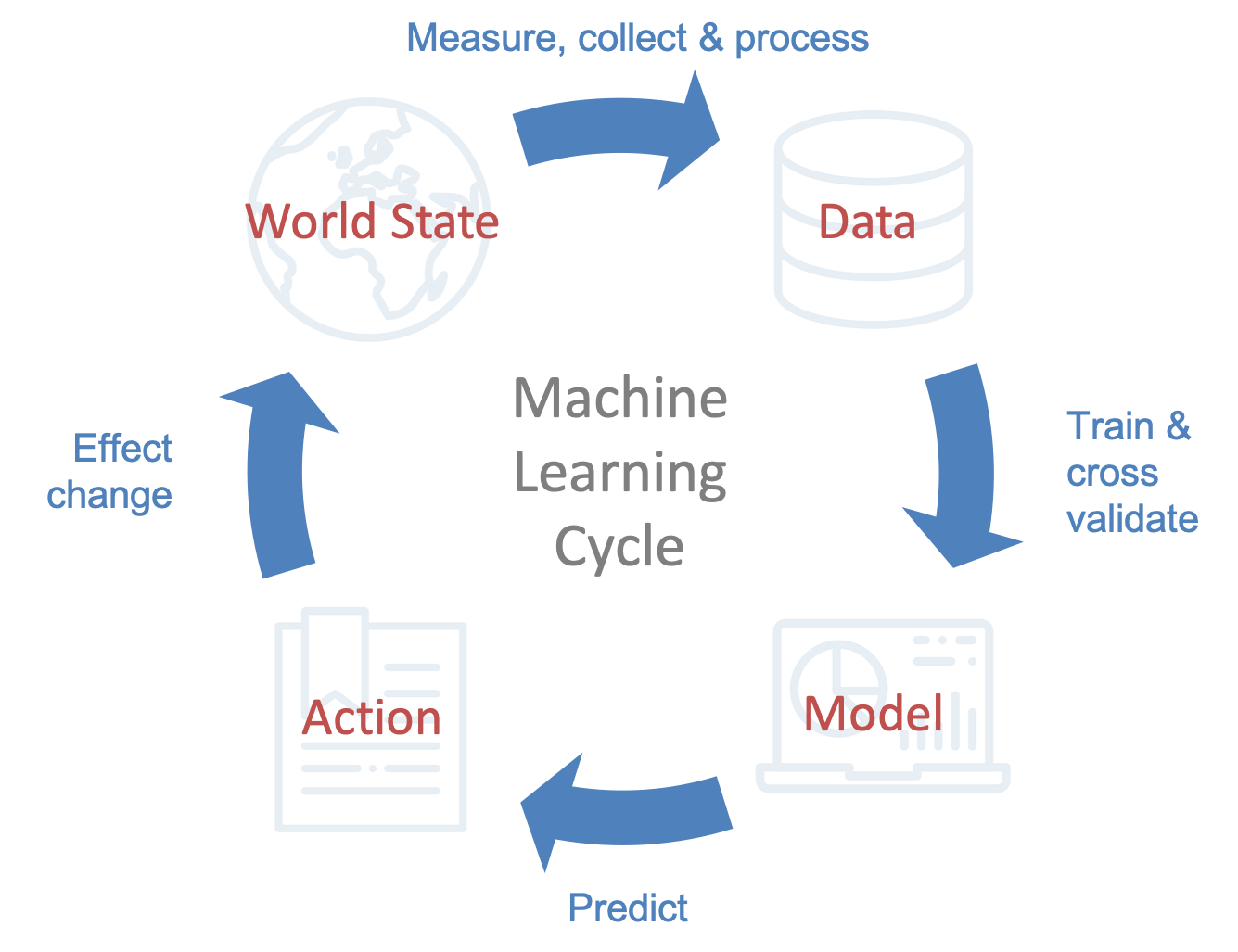
Machine learning systems can have long-term and compounding effects on the world around us. In this section we analyse the impact in a variety of different examples to breakdown the mechanisms that determine the nature and magnitude of the effect. In Figure 2.1, we present the machine learning cycle - a high-level depiction of the interaction between a machine learning solution and the real world. A machine learning system starts with a set of objectives. These can be achieved in a myriad of different ways. The translation of these objectives, into a tractable machine learning problem, consists of a series of subjective decisions; what data we collect to train a model on, what events we predict, what features we use, how we clean and process the data, how we evaluate the model and the decision policy are all choices. They determine the model we create, the actions we take and finally the resulting cycle of feedback on the data.
The most familiar parts of the cycle to most developers of machine learning solutions are on the right hand side; processing data, model selection, training and cross validation and prediction. Each action taken on the basis of our model prediction creates a new world state, which generates new data, which we collect and train our model on, and around it goes again. The actions we take based on our model predictions define how we use the model. The same model used in a different way can result in a very different feedback cycle.
Notice that the world state and data are distinct nodes in in the cycle. Most machine learning models rely on the assumption that the training data is accurate, rich and representative of the population, but this is often not the case. Data is a necessarily subjective representation of the world. The sample may be biased, contain an inadequate collection of features, subjective decisions around how to categorise features into groups, systematic errors or be tainted with prejudice decisions. We may not even be able to measure the true metric we wish to impact. Data collected for one purpose is often reused for another under the assumption that it represents the ground truth when it does not.
2.1.1 Feedback from Model to Data
In cases where the ground truth assignment (target variable choice) systematically disadvantages certain classes, actions taken based on predictions from models trained on the data can reinforce the bias and even amplify it. Similarly, decisions made on the basis of results derived from machine learning algorithms, trained on data that under or over-represents disadvantaged classes, can have feedback effects that further skew the representation of those classes in future data. The cycle of training on biased data (which justifies inaccurate beliefs), taking actions in kind, and further generating data that reinforces those biases can become a kind of self-fulfilling prophecy. The good news is that just as we can create pernicious cycles that exaggerate disparities, we can create virtuous ones that have the effect of reducing them. Let’s take two illustrative examples.
Predictive Policing
In the United States, predictive policing has been implemented by police departments in several states including California, Washington, South Carolina, Alabama, Arizona, Tennessee, New York and Illinois. Such algorithms use data on the time, location and nature of past crimes, in order to determine how and where to patrol and thus improve the efficiency with which policing resources are allocated. A major flaw with these algorithms pertains to the data used to train them. It is not of where crimes occurred, but rather where there have been previous arrests. A proxy target variable (arrests) is used in place of the desired target variable (crime). Racial disparities in policing in the US is a well publicised problem. Figure 2.2 demonstrates this disparity for policing of drug related crimes. In 2015, an analysis by The Hamilton Project found that at the state level, Blacks were 6.5 times as Whites to be incarcerated for drug-related crimes[29] [29] “Rates of drug use and sales, by race; rates of drug related criminal justice measures, by race.” The Hamilton Project, 2015. despite drug related crime being more prevalent among Whites. Taking actions based on predictions from an algorithm trained on arrest data will likely amplify existing disparities between under and over-policed neighbourhoods which correlate with race.
![Figure 2.2: Rates of drug use and sales compared to criminal justice measures by race[29].](02_EthicalDevelopment/figures/Fig_RatesDrugUseSaleRace.png)
Car insurance
As a comparative example, let’s consider car insurance. It is well publicised that car insurance companies discriminate against young male drivers (despite age and gender being legally protected characteristics in the countries where these insurance companies operate) since statistically, they are at higher risk of being involved in accidents. Insurance companies act on risk predictions by determining the price of insurance at an individual level - the higher the risk, the more expensive the cost of insurance. What is the feedback effect of this on the data? Of course young men are disadvantaged by having to pay more, but one can see how this pricing structure acts as an incentive to drive safely. It is in the drivers interest to avoid having an accident that would result in an increase in their car insurance premiums. For a high risk driver in particular, an accident could potentially make it prohibitively expensive for them to drive. The feedback effect on the data would be to reduce the disparity in incidents of road traffic accidents among high and low risk individuals.
Along with the difference in the direction of the feedback effects in the examples given above, there is another important distinction to be made in terms of the magnitude of the feedback effect. This is related to how much control the institution making decisions based on the predictions, has over the data. In the predictive policing example the data is entirely controlled by the police department. They decide where to police and who to arrest, ultimately determining the places and people that do (and don’t) end up in the data. They produce the training data, in its entirety, as a result of their actions. Consequently, we would expect the feedback effect of acting on predictions based on the data to be strong and capable of dramatically shifting the distribution of data generated over time. Insurance companies by comparison, have far less influence over the data (consisting individuals involved in road traffic accidents). Though they can arguably encourage certain driving behaviours through pricing, they do not ultimately determine who is and who is not involved in a car accident. As such, feedback effects of risk-related pricing in car insurance are likely to be less strong in comparison.
Risk related pricing and discrimination
Do you think age and gender based discrimination in car insurance are fair? Why?
2.1.2 Model Use
We’ve seen some examples illustrating how the strength and direction of feedback from models to (future) data can vary. In this section we’ll demonstrate how the same model can have a very different feedback cycle depending on how it is used (i.e. the actions that are taken based on its predictions). A crucial part of responsible model development and deployment then should be clearly defining and documenting the way in which a model is intended to be used and relevant tests and checks that were performed. In addition, considering potential use cases for which one might be tempted to use the model but for which it is not suitable and documenting them can prevent misuse. Setting out the specific use case is an important part of enabling effective and focused analysis and testing in order to understand both its strengths and weaknesses.
The idea that the use case for a product, tool or model should be well understood before release; that it should be validated and thoroughly tested for that use case and further that the potential harms caused (even for unintended uses) should be mitigated is not novel. In fact, many industries have safety standards set by a regulatory body that enshrine these ideas in law. The motor vehicle industry has a rich history of regulation aimed at reducing risk of death or serious injury from road traffic accidents that continues to evolve today. In the early days, protruding knobs and controls on the dash would impale people in collisions. It was not until the 1960s that seatbelts, collapsing steering columns and head restraints became a requirement. Safety testing and requirements have continued to expand to including rear brake lights, a variety of impact crash tests, ISOFIX child car seat anchors among others. There are many more such examples across different industries but it is perhaps more instructive to consider an example that involves the use of models.
Let’s look at an example in the banking industry. Derivatives are financial products in the form of a contract that result in payments to the holder contingent on future events. The details, such as payment amounts, dates and events that lead to them are outlined in the contract. The simplest kinds of derivatives are called vanilla options; if at expiry, the underlying asset is above (call option) or below (put option) a specified limit, the holder receives the difference. In order to price them one must model the behaviour of the underlying asset over time. As the events which result in payments become more elaborate, so does the modelling required to be able to price them, as does the certainty with which they can be priced. In derivatives markets, it is a well understood fact that valuation models are product specific. A model that is suitable for pricing a simple financial instrument will not necessarily be appropriate for pricing a more complex one. For this reason, regulated banks that trade derivatives must validate models specifically for the instruments they will be used to price and document their testing. Furthermore they must track their product inventory (along with the models being used to price them) in order to ensure that they are not using models to price products for which the are inappropriate. Model suitability is determined via an approval process, where approved models have been validated as part of a model review process to some standard of due diligence has been carried out for the specified use case.
Though machine learning models are not currently regulated in this way, it’s easy to draw parallels when it comes to setting requirements around model suitability. But clear consideration of the use case for a machine learning model is not just about making sure that the model performs well for the intended use case. How a predictive model is used, ultimately determines the actions that are taken in kind, and thus the nature of the feedback it has on future data. Just as household appliances come with manuals and warnings against untested / inappropriate / dangerous uses, datasets and models could be required to be properly documented with descriptions, metrics, analysis around use case specific performance and warnings.
It is worth noting that COMPAS[30] [30] J. Larson, S. Mattu, L. Kirchner, and J. Angwin, “How we analyzed the COMPAS recidivism algorithm,” ProPublica, 2016. was not developed to be used in sentencing. Tim Brennan (the co-founder of Northpointe and co-creator of its COMPAS risk scoring system) himself stated in a court testimony that they “wanted to stay away from the courts”. Documentation[31] [31] Northpointe, Practitioners guide to COMPAS core. 2015. for the software (dated 2015 two years later) describes it as a risk and needs assessment and case management system. It talks about it being used “to inform decisions regarding the placement, supervision and case management of offenders” and probation officers using the recidivism risk scales to “triage their case loads”. There is no mention of its use in sentencing. Is it reasonable to assume that a model, developed as a case management tool for probation officers could be used to advise judges with regards to sentencing? Napa County, California, uses a similar risk scoring system in the courts. There a Superior Court Judge who trains other judges in evidence-based sentencing cautions colleagues in their interpretation of the scores. He outlines a concrete example of where the model falls short. “A guy who has molested a small child every day for a year could still come out as a low risk because he probably has a job. Meanwhile, a drunk guy will look high risk because he’s homeless. These risk factors don’t tell you whether the guy ought to go to prison or not; the risk factors tell you more about what the probation conditions ought to be.”[30]
Propublica’s review of COMPAS looked at recidivism risk for more than 10,000 criminal defendants in Broward County, Florida[32] [32] J. Larson, “ProPublica analysis of data from broward county, fla.” ProPublica, 2016. . Their analysis found the distributions of risk scores for Black and White defendants to be markedly different, with White defendants being more likely to be scored low-risk - see Figure 2.3.
![Figure 2.3: Comparison of recidivism risk scores for White and Black defendants[32]](02_EthicalDevelopment/figures/Fig_Propublica.png)
Comparing predicted recidivism rates for over 7,000 of the defendants with the rate that actually occurred over a two-year period, they found the accuracy of the algorithm in predicting recidivism for Black and White defendants to be similar (59% for White and 63% for Black defendants), however the errors revealed a different pattern. They found that Blacks were almost twice as likely as Whites to be labelled as higher risk but not actually re-offend . The errors for White defendants were in the opposite direction; while being more likely to be labelled as low-risk, they more often went on to commit further crimes. See Table 2.1.
| Error type | White | Black |
|---|---|---|
| Labelled Higher Risk, But Didn’t Re-Offend | 23.5% | 44.9% |
| Labelled Lower Risk, But Did Re-Offend | 47.7% | 28.0% |
How might different use cases for the model affect the feedback cycle? Let’s consider some different use cases.
In the courts, the COMPAS recidivism risk score has been used by judges as an aid in determining sentence length - the higher the risk, the longer the sentence. Of course being incarcerated limits ones ability to reoffend but unless the sentence is life, release is inevitable. What impact does a longer sentence have on recidivism? Current research suggests that “The longer and harsher the prison sentence – in terms of less freedom, choice and opportunity for safe, meaningful relationships – the more likely that prisoners’ personalities will be changed in ways that make their reintegration difficult and that increase their risk of re-offending”[33] [33] C. Jarrett, “How prison changes people,” BBC Future, May 2018. . Now in addition to this consider that as a Black defendant, you are more likely to be incorrectly flagged as high risk. If there was no racial disparity in recidivism rates in the data, we could expect the imbalance in errors to create one. What about crime rates - how do longer sentences impact those? Research shows that it is the certainty, rather than severity of punishment that acts as a deterrent to crime[34] [34] D. S. Nagin, “Deterrence in the twenty-first century: A review of the evidence,” Crime and Justice, vol. 42, May 2018. . Long-term sentences are particularly ineffective for drug crimes as drug sellers are easily replaced in the community[35] [35] M. Mauer, “Long-term sentences: Time to reconsider the scale of punishment,” The Sentencing Project, 2018. . On balance, excessive incarceration has negative consequences for public safety because finite resources spent on prison are diverted from policing, drug treatment, preschool programs, or other interventions that might produce crime-reducing benefits.
Reducing incarceration rates
The US has the highest rate of incarceration in the world, at 0.7% of the population[36] [36] P. Wagner and W. Sawyer, “States of incarceration: The global context,” Prison Policy Initiative, 2018. . It’s higher than countries with authoritarian governments, those that have recently been locked in civil war and those with murder rates more than twice that in the US. Comparing with countries that have stable democratic governments, the incarceration rate in the US is more than 5 times that of its closest peer - the UK. The US spends $57 billion a year on housing more than 2.2 million people in prison[37] [37] B. Lufkin, “The myth behind long prison sentences,” BBC Future, May 2018. , almost half of which are private companies that spend significant sums on lobbying the federal government for policies that would further increase incarceration. Some have advocated for the use of risk scores in sentencing in order to reduce the rate of incarceration, the idea being that if the risk scores are low then defendants can be spared prison time. What might the feedback effect be for this use case? What is the impact of the imbalance in error rates? What assumptions are you making to reach this conclusion?
Alternatively, suppose the software was used as a way to distribute limited rehabilitation resources, allocating them to those defendants that that were deemed to be at the highest risk of re-offending (and thus the most in need of intervention). Assuming the model to be accurate and that rehabilitation decreased the risk of reoffending, we can expect that using this model would serve to reduce existing disparities in recidivism rates between individuals. What about the imbalance in errors? Black defendants would more often erroneously be allocated rehabilitation resources and white defendants erroneously denied.
We have made numerous assumptions in our analysis of the feedback above; rehabilitation consistently reduces the risk of recidivism (regardless of the crime), that the relationship between sentence length and recidivism risk is monotonic and increasing. That two years is a long enough time horizon to consider. Without getting into the weeds, the point here is simply that the same model can have a very different feedback cycle if used in a different way. How a model is used is important and its performance cannot be evaluated in isolation from its use case. A question to ask is, does the action taken on the back of the model serve to push extremes to the centre, or push them further apart? The relationships you have to understand to answer the question, will depend on the specifics of the problem.
2.2 Model Development and Deployment Life Cycle
In this section we cover the more practical aspects of ethical model development and deployment. We take a take a higher level view of the process by which machine learning systems are created and identify the stages at which we can build in safety considerations. We take inspiration from model risk management in finance where models are ubiquitous. In banking, processes and policies with regard to development, testing, documentation, review, monitoring and reporting of model related valuation risk, have been developed over decades, alongside regulation. Many of the ideas we discuss in this chapter were developed and implemented after the 2008 credit crisis in an effort to improve controls around valuation model risk for derivative products (more on this later).
Before we think about identifying and categorising common causes of harm in machine learning applications, it will be helpful to outline the workflow through which machine learning models might be developed and deployed responsibly. Figure 2.4 does exactly this.
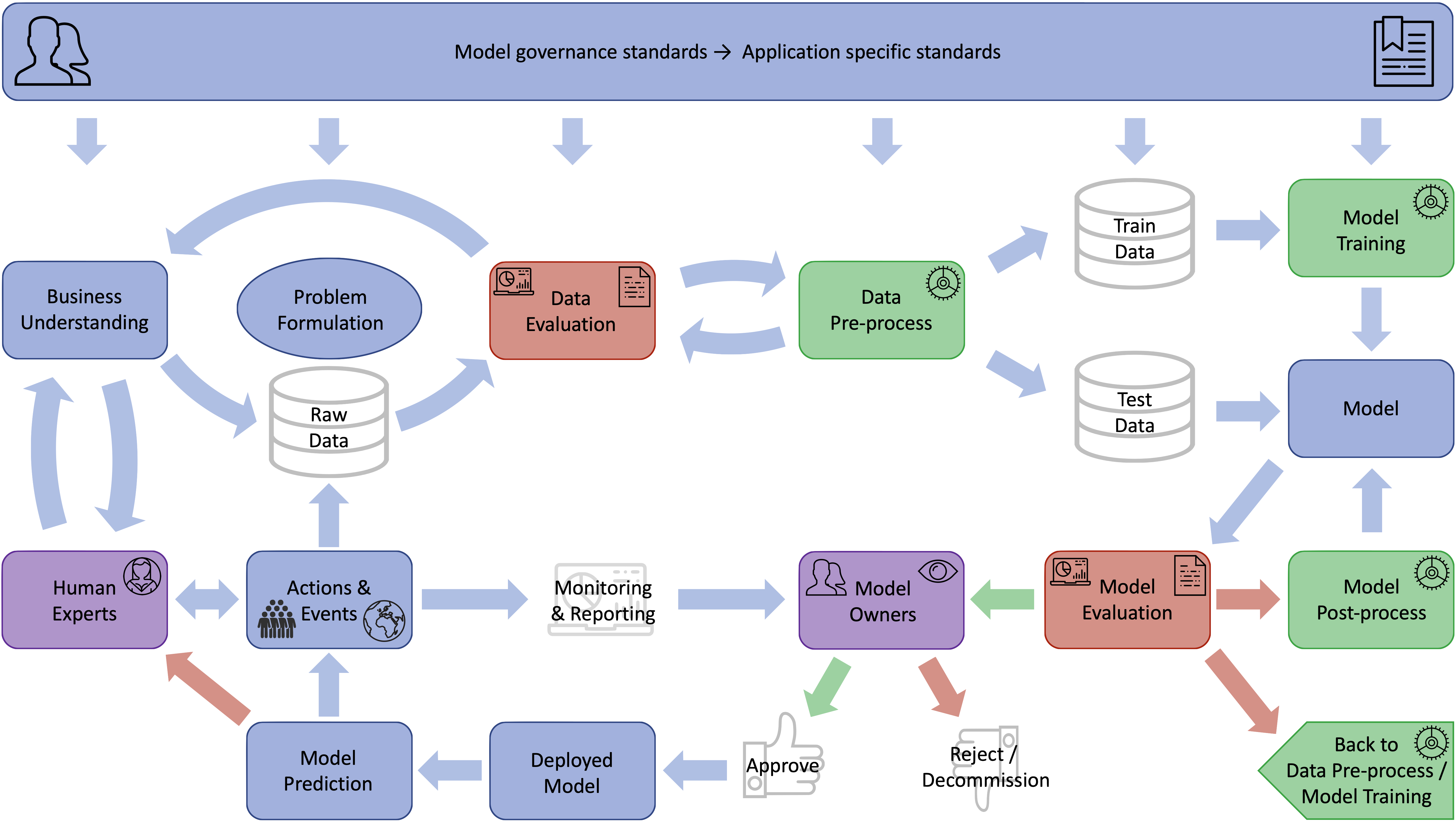
2.2.1 Model Governance Standards
At the top, overarching the entire workflow, we have the model governance standards. These essentially outline the processes, roles and responsibilities that constitute the development, deployment and management of the machine learning system. It defines and documents a set of standards for the activities that constitute each stage of the depicted workflow. More on this later.
2.2.2 Problem Formulation
Below this, the life cycle of a machine learning system starts in top left corner with the formulation of the problem. This segment of the development process includes setting objectives, gathering data, analysing and processing it, determining a target variable, relevant features and metrics that indicate success (and failure) of the model (in training, evaluating and monitoring the deployed model). This process should include consulting with experts in the problem domain. The goal here is to understand the problem, data and impact of potential solutions for all the stakeholders. The arrows show that the problem formulation process is an iterative one where ideally domain experts, data collection and processing all inform each other in the creation of a tractable machine learning problem.
An assessment should be made with regards to how appropriate the data is for the model use case. Understanding the provenance of the data (who collected it, how it was collected and for what purpose) is important. Is it representative of the population the model built on it intends to serve? Exploratory data analysis (EDA) should include understanding if there is bias and or discrimination in the data. In particular understanding how is the target variable distributed for different subgroups of the population and what the nature of the resulting machine learning cycle might be for the intended and unintended use cases. Is there strong correlation between protected features and other variables?
Problem formulation should also consider the proposed materiality of the associated risk. What’s the worst that can happen? How might the model be misused of misinterpreted? Would a disclaimer (what this model doesn’t tell you...) be appropriate? How many individuals would be exposed to the model? Is the model within risk appetite (as defined in the model governance standards)? Having a way to understand and compare the risks posed by different models/applications is useful in ensuring the appropriate amount of resource and scrutiny is applied at all stages of the development, deployment and maintenance life cycle.
2.2.3 Model Development
Once the problem is well understood and represented in the data the next broad segment is developing a model. This includes splitting the data into training and testing sets, evaluating the model against its objectives and consequently refining the data, model, evaluation metrics or other aspects. The splitting of data may be more complex, depending on the cross validation approach, but for simplicity we omit specific details in Figure 2.4. Part of model development and validation process should be to understand the model’s limitations - where predictions might be unreliable, what it can and cannot be used for. The process of testing and analysing model output for performance should include analysis for discrimination and fairness. How are predictions and errors distributed for different subgroups of the population? How does the model output distribution differ from the training data? Again, model development is an iterative process and the data, metrics, training objectives, post-processing steps and more will evolve as the developers’ understanding of the problem improves.
2.2.4 Model Owners
For applications deemed ready for deployment, the documentation for the data and model analysis and implementation is submitted to the model owners for review. So who are these model owners? There are often many people involved in the development and deployment of a machine learning system (one would hope, at least two in general) and the model governance standards should specify which of them plays what role in deciding when a solution is ready to be deployed. Each of the model owners will have different (potentially conflicting) concerns. Model owners represent the different stakeholders of the risk associated with the model and collectively they are accountable, though for potentially differing aspects of it. These might include for example,
Product owners that will use the system to make decisions.
Domain experts that may have had input in the development of the solution (legal, domain or application specific council) and/or may be responsible for dealing with cases for which the model is deemed inappropriate (a radiologist for a pneumonia detector for example).
Model developers that were involved in the construction of the model from collecting the data to building the model.
Independent model validators that provide adversarial challenge around the modelling and implementation.
Engineers that might be responsible for ensuring that infrastructure (for example, data collection, storage, post-deployment monitoring and reporting) requirements can be met.
2.2.5 Approval Process
Together model owners determine if the model is approved for deployment or not. For the sake of brevity, and to emphasize the right of the model owners to reject proposed solutions, we describe the situation where the model is not approved, as it being rejected. In reality, rejecting a model need not mean that it is scrapped. Model owners may for example require further analysis or other changes to be made before it is resubmitted for approval. In any organisation, ideally the values, mission and objectives are well enough understood by the members, that a solution being scrapped at the last hurdle would be a rare event. The kinds of issues that would result in rejection should generally be caught at an earlier stage of the model development workflow. Model owners will also be responsible for monitoring the model post-deployment, periodic re-review of the risks and failure postmortems that determine what changes are required when issues arise, including amendments to the model governance standards themselves. The model governance standards might be interpreted as a contract between the model owners that describes their commitments, individually and collectively in managing the risk.
2.2.6 Management of Deployed Models
Ensuring the necessary reporting mechanisms are in place so the decision system can be monitored both for validity and exposure, should be a pre-deployment requirement. This kind of risk tracking can be used as a control, if say limits can be defined which reflect risk appetite. Limits might be set based on how well understood the risks associated with a product (the longer a model is monitored, the more information we have about it) are and what mitigation strategies might be in place, for example.
Importantly the post-deployment cycle of Figure 2.4 (like the machine learning cycle in Figure 2.1, at the start of the chapter) includes separate nodes for the model predictions and actions taken. Selbst et al.[38] [38] A. D. Selbst, D. Boyd, S. A. Friedler, S. Venkatasubramanian, and J. Vertesi, “Fairness and abstraction in sociotechnical systems,” in Proceedings of the conference on fairness, accountability, and transparency, 2019, pp. 59–68. doi: 10.1145/3287560.3287598. , describe five traps that one might fall into, even while attempting to create fair machine learning applications. In particular, they describe the framing trap, in which one might unwittingly ensure that an algorithm meets some narrow fairness criterion on outcomes or errors (over the algorithmic frame) but fail to consider its impact in the real world. For example, failing to be sufficiently transparent about the weaknesses of it which leads to it erroneously being prioritised over the judgement of human experts. Or we might fail to consider the longer term impacts on the sociopolitical landscape (over the sociotechnical frame) in determining something as complicated as fairness. If the actions taken off the back of the predictions include human judgement or interpretation, this should also be captured as part of monitoring the model. Are people using the model in ways that were not anticipated or is it having an adverse affect in some other way? Finally we include human experts in the loop again at the stage where predictions are acted upon. Human experts might for example be consulted in cases where the model is understood to produce less reliable predictions, or via an appeals process that is built into the decision system.
Processes and procedures for managing remedial work in the event of failures could be specified as part of the model governance standards. One of the issues with machine learning solutions is that when there are failures (say, a photo or sentence is labelled in an offensive way), the easiest response is an ad hoc rule based approach to ‘fixing’ the specific issue that occurred - the “if this, then do something else” solution, so to speak. But this kind of action isn’t sufficient to address the root of the problem. Remedial work will typically require more resource and planning to fix. A failure should prompt a re-review. Having a more robust process around dealing with failures when they occur, should mean that not only is action is taken in a timely manner, but also that meaningful changes are made as a result of them and that work is appropriately prioritised.
Failure post-mortems that focus on understanding the weaknesses of the model governance process (not the failure of individuals) could also be a means for improving them. Once in production, periodic re-reviews of the model are a means to catch risks that may have been missed the first time around. The frequency of re-reviews can depend on the risk level of the model/application in question if these are being tracked.
2.2.7 Measuring Fairness
Bias and fairness metrics are essentially calculated on data. There are two stages at which we’ll be interested in measuring bias and or fairness in evaluating our machine learning system. The relevant nodes are coloured red in Figure 2.4.
Model input: The training data, during the data evaluation stage.
Model output: The predictions produced by our model, that is the model evaluation stage.
Our chosen fairness evaluation metrics calculated on the training data and model output will in general not be the same. By comparing the two, we can evaluate how well the model is replicating relationships in the data.
2.2.8 Bias Mitigation Techniques
There are three stages at which one can intervene in the development of machine learning model mapping to mitigate bias and they are categorised accordingly. Relevant nodes coloured green in Figure 2.4.
Pre-processing techniques modify the historical data on which the model is trained (at the data pre-process stage).
In-processing techniques alter the training process or objective (at the model training stage).
Post-processing techniques take a trained model/s and modify or combine the output (at the model post-process stage).
2.3 Responsible Model Development and Deployment
In this section we examine a fairness aware development, deployment and management policies for a sociotechnical system. For the most part, the ideas are similar to those concerned with effective model risk management; one that acknowledges that models are fallible and accordingly sets standards for development, deployment, monitoring and maintenance. The intention being, to prevent foreseeable failures and mitigate the associated risks. The main difference is that we consider ethical risk as a central component of the risks that must be managed. Of course predictive performance is an important consideration in being fair (it’s hard to imagine a model that is no better than guessing in making material decisions for people, as being fair) but predictive performance does not guarantee fairness. Viewing model evaluation through an ethical lens requires a more holistic assessment of the system, it’s purpose, reliability and impact; not just for the business, but for all those exposed to or affected by it - society at large.
We’ll address some of the problems that can’t be solved through the kinds of model mapping interventions we’ll talk about in this book. Another fair machine learning trap described by Selbst et al.[38] is the formalism trap, in which one fails to account for the full meaning of complex social concepts, such as fairness, which can’t be formalised with mathematical equations. In chapter 3 we’ll show that under such formalisms, a universally fair classifier is precluded by irreconcilable definitions. Fairness might more naturally be established procedurally (as often it is in law). Furthermore, social concepts are deeply contextual, and thus do not lend themselves well to abstraction (a core principal in mathematics which enables portability of solutions). Social concepts evolve over time, as cultural norms shift, therefore contestability is key, as it provides an avenue for change and challenge. These are qualities of a system rather than an equation and cannot be resolved through algorithmic interventions. They require people to do the right thing, and for organisations to define what they consider the right thing to be.
2.3.1 Policy
In industry, where innovation demands taking risks and time is money, how do we ensure the proper amount of care and attention is applied when creating products that have the potential for harm? Historically, the answer has been to impose rules that slow the process down, by requiring steps which prioritise safety over other concerns. In order to do this, one must first determine and define a safety standard. In Figure 2.4, overarching the whole process is a set of model governance standards. These essentially define that standard. They describe the process through which systems are developed and approved for deployment, and the standard to which systems are tested and evaluated.
In the financial sector, major banks (that are considered to be of systemic importance to a nations financial stability) are subjected to greater scrutiny by the central bank and regulators. An example of this might be requiring them to publish results of solvency stress tests. The currency might be social rather than financial for sociotechnical systems but the principal should be the same.
Prioritisation
Products which are of systemic importance to the sociopolitical landscape should have sufficient and appropriate resources (relative to those of the risk generating activities) to manage and mitigate their ethical risk. For applications that carry high risk of harm, risk functions should act as gatekeepers for model deployment and use.
Model governance standards
Though relatively new terminology in machine learning circles, the concept of model governance has existed for decades. For large financial institutions (which depend on vast numbers of proprietary models), operating and maintaining a model governance framework is a central part of model risk management and a regulatory requirement. The regulatory landscape of the financial sector is considerably more mature than that of other industries and the frameworks used to handle the associated risks have been developed and refined over time. It is therefore instructive to look at how such institutions manage their model risk and consider how these might be applied to sociotechnical systems.
So what does responsible and ethical machine learning development and deployment look like? In reality there is no one size fits all answer. As we’ve noted before, sociotechnical systems are context dependent. The answer can depend on a whole multitude of factors.
Domain: Different domains will have different legal and ethical concerns for example employment versus say social media.
The number and complexity of the models being used by the business: A large organisation that uses or tests hundreds of models and composes them to make decisions and create new products (such as Microsoft) would benefit greatly from infrastructure and methodologies for measuring the materiality of the associated risks that would enable prioritisation of work related to mitigating them. In contrast, for a business based on a single model that automates a specific task (such as tagging images), this would be less of a concern.
Cost of errors: Where the stakes are high, for example self driving cars, pre-deployment testing will need to be extensive and prescribed in order to reduce the probability of making mistakes. Well defined and mandatory processes will play an important role - checklists, contingency planning, detailed logging for postmortems and more. For these types of applications we would want authority over model use to be distributed to risk functions which determine when the product is approved for deployment and have the power to decommission them. For a wake word detector (think "Hey Siri", "Okay Google" and "Alexa") a lower standard would be accepted by most.
Given this, how does one approach the problem of responsible development? Step zero is to create a set of model governance standards, the purpose of which is to clearly define and communicate what responsible model development and deployment looks like for your specific application, use case, domain, business, principles and values.
What are the kinds of questions we might want our model governance standards to answer?
Why is the work important? What kinds of events or uses of your models are you trying to avoid (or are outside of the organisation’s risk appetite)? What legislation is the company subject to? What are the consequences of failures? What are the values of the company that you want to protect?
Who is responsible? What are the roles that must be fulfilled to deploy monitor and manage the risks. Who are the stakeholders or model owners and what is their remit? Who is accountable?
What are model owners responsible for? What technology is covered by the standard. What kind of expertise are required to be able to report, understand and manage the risks? What are the questions each stakeholder must answer? What are the responsibilities of those experts at the various stages of the model development and deployment life cycle? What authority do they have in relation to determining if the model is fit for deployment? Who decides what?
How do you manage the risk? What are the rules, processes and requirements that ensure the companies values are maintained, people are treated fairly, the legal requirements are fulfilled and risks are appropriately managed? How do the stakeholders work together? For example some roles might need to be independent while others work alongside one another. What are the requirements around training data (documentation, review, storage, privacy, consent and such)? What are the requirements around modelling (documentation, testing, monitoring and such)? What are the processes around proposing, reviewing, testing, deploying, monitoring model related risks? For example, frequency of risk reviews, forums for discussion and monitoring. What are the processes and requirements in place for (specific foreseeable types of) failures? Are there stakeholder specific templates or check-lists that ensure particular questions get answered at specific points in the model development and deployment life cycle?
The list of questions above is by no means exhaustive but a good starting point. Creating a set of model governance standards is about planning. Machine learning systems can be complicated and have many points of failure: problem formulation, data collection, data processing, modelling, implementation, interpretation. The only way to reduce the risk of failures is to be organised, deliberate and plan for them. Creating a set of standards does exactly that. Where the systems we build have real world consequences, the preparation, planning and process around development, review, analysis, deployment and monitoring of them should reflect that. Ensuring that the right questions get asked at the right time, knowing who is responsible for answering them and being prepared to address problems is a core part of developing and deploying models ethically.
Finally, we note that the benefits of having excellent model governance standards with well defined goals, processes, roles and responsibilities won’t be realised if in practice they are not followed. In large organisations, consistency can be a challenge. The role of internal audit is to provide objective feedback on the risks, systems, processes and compliance at an executive level. From a model governance perspective the role of auditors is to ensure that there are good processes in place and that the processes are being followed. Internal audit’s role is independent of the business up to the executive level. All functions within the business are required to cooperate with internal auditors and provide unfettered access to information requested. Internal audit does not contribute to the improvement of or compliance to processes directly. Their role is to , assess and report back to senior leadership. In a risk management context, internal audit are considered to be the third line of defence. We shall come to the first and second lines shortly.
Risk Assessment
In order to manage risk it must be identified. Any algorithm, no matter how simple, carries the risk of implementation errors or bugs and thus should at the very least be subject to unit testing and independent code review before being deployed. For organisations with more complicated risk profiles, an important component of managing risk is having a system to measure and track it. Having a way to compare risk level across products and or product classes, even if comparisons are coarse, enables some degree of risk appropriate prioritisation and resource allocation in managing them. Risk can be estimated in many different ways and exactly how it is measured will depend on the details of the application. Broadly speaking it should consider both the severity of the event and likelihood. What’s important is not the exact value but rather the ability to compare risks across products, applications or indeed any other lines along which a business is organised. Metrics that capture things like the scale on which the model is being used, predictive performance, training data quality/representativeness, model complexity, potential for harm and more could potentially be used to coarsely judge the risk posed by different applications. Model governance standards can define risk bands or metrics if they are application specific enough.
2.3.2 Risk Controls
In this section we return to the workflow and see how the policies, discussed above, feed into the development, deployment and management of a decisions system. Problem formulation is the first key step in developing a machine learning solution and an especially pivotal one in ethical risk assessment. The problem formulation stage plays perhaps the largest role in determining what the end product will actually be. It is the stage at which the model objectives, requirements, target variable and training data are determined.
Deployment Bias
As part of problem formulation one should examine the machine learning cycle in the context of the biases in the data and consider the nature (direction and strength) of the feedback of resulting actions on future data. It’s important to consider other ways in which the model might be used (other than that intended) and understand the feedback cycle in those cases. How the model might be misused/misinterpreted? Are there ways in which it should not be used? Documenting these types of considerations is an essential step in preventing deployment bias; that is, systematic errors resulting through inappropriate model use or misinterpretation of model results. As creators of technologies which affect society at large, documenting our work might be interpreted as a civic duty. We consider documentation to be an essential part of a dataset and model without which it is incomplete and potentially harmful. As such we classify lack of documentation as a model issue.
Repurposing data of models is a risky thing to do and is often the source of bias in models. A good example of this was uncovered by researchers from Berkeley in 2019. They discovered racial bias in an algorithm used to make important health-care determinations for millions of Americans [39] [39] Z. Obermeyer, B. Powers, C. Vogeli, and S. Mullainathan, “Dissecting racial bias in an algorithm used to manage the health of populations,” Science, vol. 366, pp. 447–453, Oct. 2019, doi: 10.1126/science.aax2342. . The algorithm was being used to identify patients that would benefit from high-risk care management programs, which improve patient outcomes and reduce healthcare costs for patients with complex healthcare needs. The researchers found that Black patients who had the same risk scores as White patients were far less healthier and thus less likely to be selected for the programs. The bias was the result of data documenting healthcare costs being used to predict healthcare needs.
A thorough examination of ethical issues demands consideration of a diversity of voices, which is well known to be lacking in technology. This is the stage at which it is important to consider who is affected by the technology, consult with them and ensure their views are incorporated in the understanding of the problem and design of a potential solution. Who are the human experts? People who would have valuable insight and opinions on the potential impact of the model you plan on building? Who does the model advantage and who does it disadvantage? Want to use machine learning to help manage diabetes? What are the interests of the health insurance company funding the development? Have you consulted with diabetics in addition to specialist physicians? What are their concerns? What is the problem from the different perspectives? Would a model be able to help or are there simpler solutions?
Independent Model Validation
In any system that is vulnerable to costly errors, unit testing and pre-deployment independent review is a well established method of preventing costly foreseeable failures. Whether it’s a completely new solution built from scratch or a modification to an existing solution that’s being deployed, an independent review process is an important element of responsible model development. Below we describe the responsibilities of two separate roles, the model developers and the model validators.
The model developers role is to translate the business problem into a tractable machine learning problem and create a solution. They will work with the business and receive input from other necessary domain experts relevant to the application to develop a possible solution. This will include tasks such as acquiring and interpreting data that is relevant for the problem, determining a target variable, model objectives, performance measures, fairness measures and more. In terms of preventing failures, model developers are considered the first line of defence. The responsibility of developing a model responsibly lies, in the first instance, with them. The model developers should aim to create a model they believe to be production ready and more specifically, fulfils the requirements specified in the model governance standards.
As part of the pre-deployment process, the model should be reviewed. Model validators will have a similar skill set to model developers but their goal is different to that of the model developers. Where the developers primary objective is to create a solution to the business problem that meets a standard which will be approved by model owners, the role of a model validator is to critique that solution and expose problems with it - the more the better. Their role is to adversarially challenge the solution. They might challenge performance claims (error, bias, fairness) by changing the data or metrics, or demonstrate problems with the model by comparing with an alternative solution. The goal is to expose model weaknesses and demonstrate the limits of its validity in testing and documentation. The model validator might devise mitigation strategies for identified risks. Such strategies might include setting model usage limits (that might trigger a re-review for example) or additional monitoring requirements. They might for example identify additional cases when human review might be required or reject the proposed solution entirely if the problems with the model are great enough. The role of the reviewer could be thought of as something akin to a hacker but with the advantage of having the keys in the form of model documentation (provided by the developers). The model reviewer in pre-deployment can act as a gatekeeper.
Note that in our terminology, the model is simply a mapping. It need not be learned by calibration to historic data. Any algorithm where the decision being made is important enough should be treated as such and proper precautions should be taken. For an algorithm which will be used in production, no matter how simple, this should mean being subject to code review and unit testing that demonstrates its validity in some well chosen cases. A good example of where this would have been valuable came up in December 2020 when a bug in an algorithm, meant that Stanford Hospital Residents were not correctly prioritised for the COVID-19 vaccine, despite working with COVID-19 patients daily. The algorithm did not apparently account for the fact that Resident doctors had a blank ‘location’ field in the data. We might never know the details of how it was implemented and tested but it hard to imagine such a bungle passed any decent unit test.
The model review process acts as the second line of defence. To be effective, the model reviewer’s role must be independent of the model developer’s to some extent. What does independence mean? We mentioned the distinct goals of their roles and this is important. The validator should not drive the development of a solution approach or model but instead focus on critique. In reality, it’s easy to see that the iterative nature of model development might mean that amendments addressing criticisms of the solution may get rolled into it’s development at multiple stages, blurring the lines between critique and collaboration. From an efficiency perspective, it might make sense for the solution to be reviewed at several critical stages of the development process making the overall process indeed more collaborative. If there’s a problem with the data that was missed, ideally the developer would want to fix it before going on to build and train a model on it. One of the challenges then is how to preserve independence between the roles, and ensure that the value of having adversarial criticism in preventing failures, is not lost in collaboration. How best to preserve independence will depend on the specifics and is something that should be determined within the model governance standards. In a bank, the model developers and validators are required (by the regulator) to serve under different business functions (the trading desk versus risk management). They have different reporting lines up to executive level, and work in physically separate locations.
Monitoring
Post-deployment monitoring is an important part of responsible model development and deployment. Analysis should not stop once the model is deployed. Decisions on what to monitor and necessary feedback mechanisms should be determined during development. It’s important to understand if the model is performing in line with expectations (based on pre-deployment testing and analysis). Is the data coming out of the model more or less biased than the data going in? Distributional shifts should be of particular concern where the actions taken based on predictions have a strong impact on the composition of future data.
Domain Expertise
In section 1.4 we spoke of the importance of domain knowledge in interpreting causal relationships in data. Consulting domain experts at the problem formulation stage can yield considerable ethical risk reducing benefits. Incorporating more diverse perspectives on a problem will surely result in a better design that will benefit a broader cross-section of society. Given that models are simplified representations of real world systems and we know that they will make errors, responsible development should build in processes for anticipating and dealing with such cases and, where appropriate, deferring to the judgement of a human expert.
2.4 Common Causes of Harm
There are many ways in which machine learning solutions can result in harm. In this section we present a taxonomy of common causes and provide examples. At the end of the section, we’ll relate the causes in our taxonomy to the corresponding stages of the model development and deployment life cycle (discussed earlier), indicating where consideration and intervention could prevent them from arising. The goal is for this to serve as a good starting point as a practical reference for developing fairer models. For practising data scientists it could be helpful as a standard to compare our current practices against, avoid common pitfalls and hopefully help ensure we perform an appropriate level of due diligence before releasing our work. In our taxonomy, we aim to layout both the points at which issues arise and the various points at which one could assess and intervene. For this reason, the table may appear to contain duplications of the same problem viewed from different perspectives. This is intentional. Often different parts of an application are developed independently.It’s not uncommon for example (thanks to unprecedented growth in data markets), for a model to be built by one organisation, based on data collected by another.
Taking this approach is beneficial since it provides multiple opportunities to see and remedy the same problems.
Before presenting this taxonomy, it’s worth being clear that, in reality, there is no agreed upon terminology that describes the different types of issues that can arise or agreed upon framework for developing machine learning solutions that factor in ethical safety concerns (since regulation surrounding algorithmic decision systems is still in the process of being shaped). Indeed, developing one is the subject of recent research, [40] [40] B. d’Alessandro, C. O’Neil, and T. LaGatta, “Conscientious classification: A data scientist’s guide to discrimination-aware classification,” Big Data, vol. 5, no. 2, pp. 120–134, 2017, doi: 10.1089/big.2016.0048. , [41] [41] H. Suresh and J. Guttag, “A framework for understanding sources of harm throughout the machine learning life cycle,” 2021. , [42] [42] T. Gebru et al., “Datasheets for datasets.” 2020.Available: https://arxiv.org/abs/1803.09010 , [43] [43] M. Mitchell et al., “Model cards for model reporting,” Proceedings of the Conference on Fairness, Accountability, and Transparency, 2019, doi: 10.1145/3287560.3287596. . The word bias itself has many definitions and even in a given context can have multiple valid interpretations. Different practitioners would likely describe the same type of bias differently. Causes of bias in machine learning applications are often numerous and overlapping, thus difficult to attribute to a single source or prescribe a single solution for. The most appropriate remedy itself will be very much context dependent and different practitioners will choose different approaches.
In creating this taxonomy, we take inspiration from that described by d’Alessandro et. al.[40], in which the model or algorithm (function mapping \(f\) from features \((\boldsymbol{X}, \boldsymbol{Z})\) to predictions \(\hat{Y}\)), is distinguished from the larger system (people, infrastructure, processes, policies and risk controls) through which it is developed, deployed and managed. Evidence based medicine provides a rich terminology for different mechanisms through which systematic errors can be introduced in data and has perhaps the most comprehensive set of definitions and classification of bias types. This in itself can provide an important reference in determining which kinds of biases model developers should be aware of and we include some of them here. Table 2.2 summarises our taxonomy of common causes of harm in machine learning systems.
| Element | Failure | Issue Type | Issue Description |
|---|---|---|---|
| System | Policy | Prioritisation | Failure to allocate appropriate/sufficient resource |
| Failure to distribute power to manage conflicts of interest | |||
| Governance | Failure to set or comply with application specific standards | ||
| Risk assessment | Failure to identify and manage model related risk | ||
| Controls | Deployment bias | Inappropriate model use / misinterpretation of model results | |
| Independent model validation | Data appropriateness and preparation | ||
| Modelling approach and implementation | |||
| Model evaluation metrics (pre and post deployment) | |||
| Monitoring | Poor monitoring of model validity and impact | ||
| Poor monitoring of risk exposure | |||
| Domain expertise | Non deference to human domain expert | ||
| Model | Data | Historical bias | Data records wrongful discrimination |
| Measurement bias | Quality of data varies across protected classes | ||
| Measurement process varies across protected classes | |||
| Recording proxies for immeasurable / ill defined variables | |||
| Representation bias | Data not representative of target population | ||
| Low support | Insufficient data for minority classes | ||
| Documentation | Failure to adequately document | ||
| Misspecification | Aggregation bias | Failure to model differences of type | |
| Target variable | Target variable subjectivity | ||
| Proxy target variable learning | |||
| Heterogeneous target variable | |||
| Features | Inclusion of protected features without control variables | ||
| Inclusion of protected feature proxies (redlining) | |||
| Cost function | Failure to specify asymmetric error costs | ||
| Omitted discrimination penalties | |||
| Evaluation bias | Poor choice of evaluation metrics | ||
| Test data not representative of the target | |||
| Documentation | Failure to adequately document |
In section 2.3 we discussed a framework for responsible development and deployment of models. We summarise important elements of that discussion under system issues in our taxonomy of harms. The idea is that if having a process in place could avoid certain types of harms, then not having them is a failure of the system surrounding the model. In this section we discuss common causes of discrimination that relate directly to the model. We categorise these as originating from failures related to one of two sources:
Data issues refer to harms that arises as a direct result of issues with the data
Misspecification refers to harms that arise through misspecification of the underlying problem in the modelling of it.
The latter is an extension of the notion of model misspecification in statistics where the functional form of a model does not adequately reflect observed behaviour.
Before discussing our taxonomy for modelling issues, we address a point of contention in the machine learning community - that models are not biased, bias comes from data. The notion that bias is simply an artifact of data rather than a model is not uncommon among machine learning scholars and practitioners. In this book we’ve already discussed numerous examples of biased machine learning models, so where does this idea come from? In more theoretical disciplines a model is interpreted as being the parametric form. Under this definition of a model, different values of the parameters then don’t change what we consider to be our model. For example, the term linear model describes a family of models. More practical disciplines view a model as a function mapping - provided with input, the model returns output. By this definition of a model, if the parameters change, so does the function and thus the model. From a practical perspective then it’s clear that a model can discriminate since if the data documents historic discrimination, we would expect the trained model to reproduce it.
The idea that bias is a data problem, rather than a modelling one is at best a gross oversimplification of the problem and at worst misleading. It implies that in general, after training, a model will perfectly reproduce the joint distribution of the variables in data. Anyone who’s ever trained a model on real world data knows, is patently false. It suggests that models and data are independent when, in practice, they ought not be. Model development is an iterative process. The modelling choices we make can depend on the data and our model results should in turn influence our training data. Treating data and modelling as independent entities diminishes the responsibility of model developers in addressing the problem of biased and unfair applications. It ignores the very practical nature of developing models and the societal impact they can have. For sociotechnical systems, the objectives must surely extend beyond utility. We consider defining those wider objectives and incorporating them part of the modelling process and thus failing to consider them a modelling problem.
2.4.1 Data Issues
When it comes to bias, data driven medicine provides a rich vocabulary for the different types. We mention three here.
Historical Bias
Historical bias arises as a result of differences between accepted societal values and cultural norms and those captured by data. These need not be a result of errors in the data. Even if data perfectly represents some world state, it can still capture a reality which society deems unfair. Training a model on such data will naturally lead to similarly unfair predictions. Historical bias can manifest itself in data in numerous ways, through unfair outcomes recorded in the data, differing data quality across groups and under or over-representation of groups to name just a few. Take medical data where racial and gender disparities in diagnosis and treatment are well publicised as the health gap. There is a growing body of research across the US and Europe that exposes systematic under-treatment and misdiagnosis of pain in women ([44] [44] K. L. Calderone, “The influence of gender on the frequency of pain and sedative medication administered to postoperative patients,” Sex Roles, vol. 23, pp. 713–725, 1990, doi: https://doi.org/10.1007/BF00289259. , [45] [45] E. H. C. MD et al., “Gender disparity in analgesic treatment of emergency department patients with acute abdominal pain,” Academic Emergency Medicine, vol. 15, pp. 414–418, May 2008, doi: https://doi.org/10.1111/j.1553-2712.2008.00100.x. , [46] [46] D. E. Hoffmann and A. J. Tarzian, “The girl who cried pain: A bias against women in the treatment of pain,” SSRN, 2001, doi: http://dx.doi.org/10.2139/ssrn.383803. ) and Black patients (despite prescription drug abuse being more prevalent among White Americans), [47] [47] K. M. Hoffman, S. Trawalter, J. R. Axt, and M. N. Oliver, “Racial bias in pain assessment and treatment recommendations, and false beliefs about biological differences between blacks and whites,” Proceedings of the National Academy of Sciences, vol. 113, no. 16, pp. 4296–4301, 2016, doi: 10.1073/pnas.1516047113. .
Measurement Bias
Measurement bias refers to non-random noise in measurements across groups. This can occur if for example, there are geographic disparities in services provided by an institution or the quantity and quality of the measuring instruments that mean the accuracy and completeness of records vary by location (and other highly correlated variables like race). In some cases institutions can systematically fail to produce accurate and timely records for certain groups. For example, in medical data, where more frequent misdiagnosis of rare diseases for women leads to a longer lag before accurate diagnosis. In particular, 12 compared to 20 months for Crohn’s disease (despite the disease being more prevalent among women) and 16 compared to 4 years for Ehlers-Danlos syndrome[48] [48] “The voice of 12,000 patients: Experiences and expectations of rare disease patients on diagnosis and care in europe.” 2009. . Systematic delays in diagnosis for protected groups mean that for any given snapshot in time, the medical records for more frequently misdiagnosed groups are less accurate.
Another way in which measurement bias can manifest is if the measurement process varies across groups, for example where the level of scrutiny varies across groups. Predictive policing discussed earlier provides an example of this where there are existing disparities in the level of policing across neighbourhoods. But in practice any process (algorithmic or otherwise) which seeks to identify a behaviour or property (good or bad), but where disproportionate attention is allocated to some subgroup will result in disproportionately more instances of that behaviour or property being observed among members of that group. The result is induced correlation in the data, even in cases where there may in reality be none. One must be careful of making the assumption that where no observation was made the behaviour or property did not exist. The result can be a cycle that continually amplifies the association. Since data often measures and records features which are in fact noisy proxies for the true variables of interest, measurement bias includes cases where use of proxies leads to systematic errors.
Representation bias
Representation bias occurs as a result of biased sampling from the target population. It can be observed as differences in the prevalence of groups when comparing the target population and the sample data. Under-represented classes are exposed to higher error rates; a problem which arises as a result of ‘low support’, that is a smaller pool of data points to train the model on. Looked at from the perspective of the majority class which dominates the aggregate error, the algorithm is naturally incentivised to focus learning characteristics of majority classes.
One of the drivers behind big data initiatives is the plummeting cost of collection and storage data. Companies and institutions are able to train models that better target individuals, reducing costs and boosting profits. However, data collection methods often fail to adequately capture historically disadvantaged classes of people that are less engaged in data generating ecosystems. A good example of this, given by Barocas & Selbst[4] is that of the phone app Street Bump, which was developed by the City of Boston to reduce the cost and time taken to find (and consequently repair) pot holes. The app uses data generated by the accelerometers and GPS of Boston residents’ smart phones as they drive. Once a pothole is located it is automatically added to the city’s system to schedule a repair. One can see easily see how this method of data collection might fail to adequately capture data from poorer neighbourhoods, where car and smart phone ownership are less prevalent; neighbourhoods which probably correlate with race and are already likely to suffer from lack of investment.
In the extreme case of under-representation, there is no support, that is to say, no data points to train on at all. This can be a problem when say studies of symptoms or clinical trials for drugs have no representation for certain groups among which symptoms or drug effectiveness may well vary. A good example of this is diabetes, the impact of the disease and effectiveness of drugs for which have historically most often been measured on samples with few to no hispanic individuals in datasets at all.
Low support
Low support may lead to undesirably high errors for some groups even in the absence of representation bias, since minority classes naturally have fewer data points to train on. This is a particular problem for individuals belonging to multiple disadvantaged classes, for example Black women, which are often overlooked when studies seek to meet fairness metric targets.
Documentation
Documentation of datasets is an essential step in avoiding data misuse or misinterpretation of variables or relationships in the data due to lack of domain knowledge. Documentation should evidence that model governance standards were met. Summaries that explain the provenance of the data (who collected the data, for what purpose, what population was sampled from and how, limitations of the data, clear explanation of the target variables (including consideration of use cases for which it would not appropriate for), breakdown of the demographics and the variables by sensitive features pointing out classes that are not well represented. Documentation that is standardised through use of a template could ensure some level of consistency.
2.4.2 Misspecification
Aggregation Bias
Aggregation bias occurs when heterogeneous groups are modelled as homogeneous. In this case we are assuming the same model is appropriate for all groups when in fact it is not, it is a failure to recognise differences in type. There are many examples of this is medical models for diagnosis or that measure the effectiveness of treatments. Historically much of medical research is based on data that over-represents White men. Diseases that manifest differently across gender or race are more often misdiagnosed or less effectively treated. Take autism spectrum disorder (AUD) for example, in 2016 research estimated that autism is four times more prevalent in boys than girls. However more recent research has suggested that a contributing factor maybe that autism more often goes undiagnosed in women because studies of the disorder have historically been focused on male subjects. The most notable difference between autistic males and females is how the social (rather than behavioural) symptoms manifest. It is thought that women, especially at the high-functioning end of the spectrum, are more likely to camouflage their symptoms.
Target Variable Selection
One of the challenges in developing a machine learning is the translation of the underlying problem by defining a target variable - something which can be observed, measured and recorded or obtained easily (from a third party vendor), and that accurately reflects the variable we wish to predict. While there are relatively uncontentious examples that machine learning solutions lend themselves well to (spam detection for emails or on-base or slugging percentage for major league baseball player valuation) for many problems the translation is non-trivial and subjective. Take a job applicant filter for example, that aims to find the most promising applicants. The attributes that one might consider to be held by an applicant that make them promising are likely to be described differently by different people even if they work in the same team. Even if two individuals agree on the attributes, it’s likely they’ll weigh the attributes differently based on their experiences and preferences. Different choices will result in the different kinds of biases infiltrating our algorithm.
Often when data on the variable we want to affect doesn’t really exist we use a proxy. In 2018, Amazon was forced to scrap a recruitment tool it spent four years developing. The algorithm rated resumes of potential employees and was trained on 10 years worth of resumes submitted by job applicants. The exact details of the algorithm were not publicised but based on the training data, it is likely that the proxy variable they used was some measure of how the candidates had performed in the hiring process previously. Thus predicting who they would have hired in the past (given their historical and existing biases) rather than who was the best applicant. The problem with such systems is that often they end up being how we define the thing that it’s actually a proxy for.
Issues can also arise when defining a heterogeneous target variable, where a range of different events are coarsely grouped into a single outcome. This is a form of aggregation bias where the issue specifically concerns the target. This might happen for example where the event of particular interest is rare and by including more events in the target the predictive accuracy of the model increases as it has more data to learn from. D’Alessandro et. al[40] provide a useful example in predictive policing where the model developer is initially interested in predicting violent crime but ends up incorporating petty crimes (which happen much more frequently) in the target variable in pursuit of a more accurate model. The model then ends up trying to learn the features of a more nebulous concept of crime ignoring important differences between different types. Another example might be building a gender recognition system and only recognising people as one of two genders[25].
Feature selection
In an ideal world we would train a machine learning model on a sufficiently large dataset consisting of a rich set of features that actually influence the target variable rather than simply being correlated to it. More often than not, the reality is rather different. Comprehensive data can be expensive and difficult to collect. Factors that influence the target variable might not be easily measured or be measurable at all, while data containing more erroneous indicators might simply be cheaper to obtain or more readily available. This is a common way in which bias against protected classes can enter our model.
The inclusion of protected features without control variables might arise because a protected feature appears to be predictive of the target variable where explanatory variables are not known or available. Of course in cases where using protected characteristics as inputs to an algorithm would lead to disparate treatment liability, this is not a problem one is typically faced with, but it’s worth reiterating the importance of controlling for confounding variables, in drawing conclusions about relationships between features from observational data (see section 1.4).
Inclusion of protected feature proxies, as is the case with redlining, is perhaps a more common problem. One where protected features are not used as inputs to the model, but features which are predictive of them are. Historically employers have taken the reputation of the university that applicants graduated from as a strong indicator of the calibre of the candidate. But many of the most reputable universities have very low rates of non-White/Asian students in attendance. A hiring process which is strongly influenced by the university from which the applicant graduated, can erroneously disadvantage racial groups that are less likely to have attended them. While the university an applicant graduated from, might correlate to some degree with success in a particular role, it is not in itself the driver. An algorithm that directly takes into account the skills and competencies required for the role would be more predictive and simultaneously less biased. Given the cost of collecting comprehensive data, one might argue that higher error rates for some classes would be financially justified (rational prejudice).
Cost function
A critical consideration in how we specify our model is the cost function. It is how we evaluate our model in training and essentially determines the model (parameters) we end up with. The cost function can be interpreted as an expression of our model objectives and so provides a natural route to addressing discrimination concerns. A common failure in the design of classification models is proper accounting of the costs of the different types of classification errors (false negative versus false positives). If the harm caused by the different types of misclassification are asymmetric, the cost matrix should reflect this asymmetry.
More broadly (for both regression and classification), it is important to consider the contribution from each sample in the training data to the cost function in training. Upsampling (or simply up-weighting, depending on the learning algorithm you are using) is a valuable tool to keep in mind and can alleviate a number of the issues discussed above, that are common sources of bias. Let’s take the issue of low support. By upsampling minority classes, one can increase the importance of reducing errors for those data points, relative to other more abundant classes, during learning. Though it’s worth noting that it cannot resolve issues relating to a lack of richness of representation for classes with low support. Another case in which upsampling can help is that discussed in relation to definition of a heterogeneous target variable. By upsampling data points that correspond to the primary event of interest (violent crime in the example we discussed above), one can again increase the importance of the model fitting to those data points.
For an algorithm that solves a problem in a regulated domain, it would make sense for the absence of discrimination to be a model objective along with utility. This can be achieved by use of a penalty term in the cost function which relates to discrimination in the resulting predictions (just as we have terms that relate to the error or overfitting). Essentially the idea is similar to that of regularisation to avoid overfitting. We introduce an additional hyper-parameter to tune, which represents the strength of the penalty for discrimination in our cost. We will discuss this and upsampling in more detail when we discuss bias mitigation techniques, in part three of the book.
Evaluation bias
Evaluation bias arises when evaluating a model’s performance. There are two main components here, the metrics chosen to describe the model’s performance and the benchmark dataset on which they are calculated. Choosing either inappropriately will result in our evaluation metric inaccurately reflecting the efficacy of our model. For sociotechnical problems in particular choosing good metrics requires domain knowledge - the wider political, legal, social and historical context is important when defining what success and failure look like. For example, if building a gender recognition system, one should not simply think of the performance on the specific task but also the wider infrastructural systems which might find the technology useful. Where should we set the bar for such a technology? That should surely depend on how the technology is used after the prediction is made? Are there controls around model use? Should there be? What kinds of risk level does the model present? What might be the impact of the prediction being incorrect? When would an error be fair? What kind of examples would you expect your system to get wrong and why? What do they gave in common? Are they represented in the benchmark dataset? By asking these kinds of questions, when deciding what success looks like, it’s hard to imagine thinking that minimising the mean squared error on a conveniently available dataset would be sufficient.
One approach might be to set accuracy thresholds across all (skin colour) phenotype and gender combinations [25]. This would be one way of thinking about success in a way that incorporates some of our societal values of equality. The gender recognition software we talked about in the previous chapter suffered from evaluation bias on both counts. The benchmark datasets used were not representative of the target population and the metrics that were chosen, failed to expose the models poor performance on darker skinned women. The problem of evaluation bias arising from poor choice of testing/benchmark data is often the result of trying to objectively compare performance across models and can lead to overfitting to said benchmark data.
Documentation
Documentation for models (as for datasets) can have a significant impact when it comes to avoiding model misuse (a model use it is not appropriate/approved for) and ensuring model limitations are well understood. It can reduce the risk of misinterpretation of variables as suitable proxies for other variables. Clear explanation of the model, testing that was performed, on what subgroups of the data can make it easier to know which tests might be missing that would offer insight into the validity of the model. Documentation should evidence that the model governance standards have been met. Descriptions of the data and model, motivation behind subjective decisions that were made to arrive at the solution (how to process the data, what features were used/ignored and why, model type, cost function, sample weights, bias and success metrics), known data/model issues, how the model was tested, what it’s limitations are, what it should and should not be used for with justification. Documentation of the model should provide enough detail to be able to re-implement the model, reproduce results and justify the solution approach. Documentation that is standardised through use of a template could ensure some level of consistency and efficiency across domains and applications. Recent research discusses the matter specifically for publicly released datasets[42] and machine learning models[43]. They suggest standardised analysis which for example demonstrates the performance of the algorithm for different subgroups of the population and requirements for proving efficacy for conjunctions of sensitive characteristics also.
2.5 Linking Common Causes of Harm to the Workflow
In Figure 2.5 we provide a visual summary of the taxonomy in Table 2.2, the goal being that it might be useful as a reference for teams developing machine learning technologies. Since failures of policy do not relate to any particular part of the model development and deployment life cycle but rather all of it, we omit these.
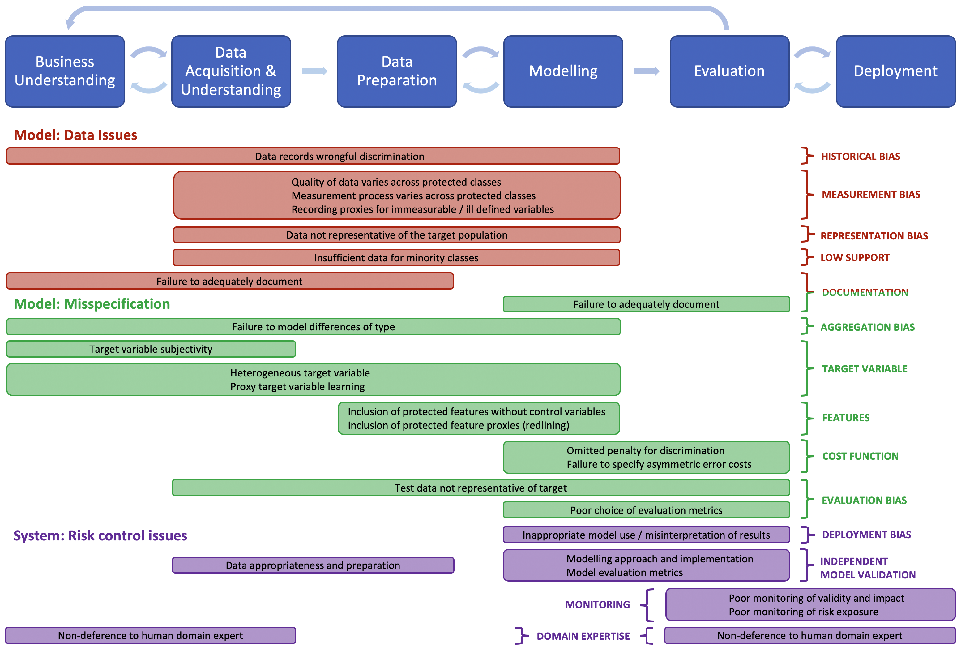
At the top of Figure 2.5 we have a simplified version of the model development and deployment life cycle. Below this, the causes of harm are displayed in boxes which span the parts of the lifecycle to which they relate. We use colour to separate different categories of failures and curly brackets to group issues by type.
Summary
Machine learning cycle
Machine learning solutions can have long-term and compounding effects on the world around us. Figure 2.1 illustrates the interaction between a machine learning solution and the real world.
The translation of a given problem and objectives into a tractable machine learning problem, requires a series of subjective choices. Choices around what data to train the model on, what events to predict, what features to use, how to clean and process the data, how to evaluate the model and what the decision policy should be will all determine the model we create, the actions we take and ultimately the cycle we end up with.
Data is a necessarily subjective representation of the world. The sample may be biased, contain an inadequate collection of features, subjective decisions around how to categorise features into groups, systematic errors or be tainted with prejudice decisions. We may not even be able to measure the true metric we wish to impact. Data collected for one purpose is often reused for another under the assumption that it represents the ground truth when it does not.
In cases where the ground truth (target variable) assignment systematically disadvantages certain classes, actions taken based on predictions from models trained on the data are capable of reinforcing and further amplifying the bias.
Decisions made on the basis of results derived from machine learning algorithms trained on data that under or over-represents certain classes can have feedback effects that further skew the representation of those classes in future data.
The actions we take based on our model predictions define how we use the model. The same model used in a different way can result in a very different feedback cycle.
The magnitude of the feedback effect will depend how much control the institution making decisions based on the predictions, has over the data the training data.
Just as we can create pernicious machine learning cycles that exaggerate disparities, we can also create virtuous ones that have the effect of reducing disparities. Therefore it’s important to consider the whole machine learning cycle when formulating a machine learning problem
Model development and deployment life cycle
Figure 2.4 depicts the model development, deployment and monitoring life cycle at a high level. Overarching the entire workflow, are the model governance standards. These essentially outline the processes, roles and responsibilities that constitute the development, deployment and management of the machine learning system. It defines and documents a set of standards for the activities that constitute each stage of the workflow.
Problem formulation: Translating a business problem into a machine learning one.
The problem formulation stage plays a pivotal role in what the end product will actually be. It is the stage at which the model objectives, requirements, target variable and training data are determined and it is the stage at which perhaps the most important ethical question (whether the model should be built at all) must be answered.
Consider who is affected by the technology, consult with them and ensure their views are understood and incorporated in the understanding of the problem and design of a potential solution.
Assess the materiality of the risk. What’s the worst that can happen? How likely is such a failure? How many people are exposed to the model?
Examine the machine learning cycle in the context of the biases in the data and consider the nature (direction and strength) of the feedback of resulting actions on future data.
Consider other ways in which the model might be used (other than that intended) and the corresponding feedback cycle in those cases. How the model might be misused?
Independent model validation: An independent review process is an important element of responsible model development. This means that pre-deployment there are two separate data science roles, model development (designing a solution) and the model validation (critical assessment of the solution).
Model development: The model developers role is to translate the business problem into a tractable machine learning problem and create a model solution.
The model developer will work with the business and receive input from other necessary domain experts relevant to the application to develop a possible solution.
The model developer should document the solution. Documentation should include descriptions of the data and model, justification of the approach, known issues and limitations, model testing (biases as well as performance), what the model should not be used for and why. Templates are a good way of standardising documentation.
In terms of preventing failures, the model developer is the first line of defence. The responsibility of developing a model responsibly and ethically lies, in the first instance, with them.
Model validation: The role of a model validator is to criticise the proposed solution.
The model validator will identify and expose issues with the problem formulation, data and data processing. They will verify the model performance metrics (error, bias, fairness), look for model weaknesses and demonstrate them through testing. They may also devise mitigation strategies for identified risks.
The role of the reviewer might be thought of as a hacker but with the advantage of having access to the model documentation (provided by the model developer). They also act as a gate keeper.
The model reviewer must also document their analysis, testing and critique and recommendations regarding the solution.
The model reviewer acts as the second line of defence.
Model approval: The model owners collectively determine if a solution is ready for deployment.
Model owners act as the final stage gate keepers before deployment. They will each have been involved in different aspects of the development and deployment of the machine learning system.
In effect, the model owners represent the different stakeholders of the risk associated with the model and collectively they are accountable, though for potentially differing aspects of it.
They will also be responsible for monitoring the model and risk materiality post-deployment and ensuring that periodic re-review, failure processes and post-mortems occur and are effective.
The model governance standards might be interpreted as a contract between the model owners that describes their commitments, individually and collectively in managing the risk.
Monitoring of deployed models: The world is dynamic and the risk associated with models evolves with it. Deployed models should be monitored to understand if they are behaving in line with expectations. The metrics which should be reported to model owners should be identified pre-deployment by the model developer and validator.
Risk materiality tracking: As model usage increases so does the associated risk. As part of monitoring, metrics that give an indication of the risk associated with the model is should be reported to the model owners.
Periodic re-review: The pre-deployment independent review of the model is just the first. Thereafter, periodic re-reviews of the model are a means to catch risks that may have been missed the first time around. The frequency of re-reviews will depend on the risk level of the model/application in question.
Failure event process: Processes and procedures in the event of failures should be specified as part of the model governance standards, in particular what steps should be taken by which model owner. Having a robust process around dealing with failures when they occur should mean that action is taken in a timely manner and that meaningful changes are made as a result of them.
Failure post-mortems: A post-mortem should focus on understanding the weaknesses of the model governance process (not the failure of individuals) that contributed to it and appropriately prioritise any changes required to remedy them.
Measuring bias: Bias and fairness metrics are essentially calculated on data; the data going into our model (training data) and the data coming out of it (the predictions produced by our model); the data evaluation and model evaluation stages.
Bias mitigation techniques: There are three stages at which one can intervene to mitigate bias when developing a machine learning model labelled data pre-process, model training and model post-process in Figure 2.4. We categorise them accordingly:
Pre-processing techniques modify to the historical data on which the model is trained, the idea being that fair/unbiased data will result in a fair/unbiased model once trained.
In-processing techniques alter the training process or objective in order to create model with fairer/less biased predictions.
Post-processing techniques take a trained model and modify the output such that the resulting predictions are fairer/less biased.
Responsible model development and deployment
Model governance standards
Machine learning systems can be complicated and have many points of failure: problem formulation, the data collection, data processing, modelling, implementation, deployment. The only way to reduce the risk of failures is to be organised, deliberate and plan for them. Creating a set of standards does exactly that. They make sure the right questions get asked at the right time and that there is clarity around who is responsible for what.
The purpose of creating a set of model governance standards is to clearly define and communicate what responsible model development and deployment looks like for your specific application, domain, business, principles and values. It essentially documents and communicates the why, who, what and how of your model risk management approach.
Why is the work important? What kinds of events are you trying to avoid? What are the consequences of failures? What are the values of the company that you want to protect?
Who is responsible? Who are the stakeholders? Who is accountable for managing the various identified risks?
What are they responsible for? What are their roles/expertise? What authority do they have in relation to determining if the model is fit for deployment?
How do you manage the risk? What are the policies, processes and requirements that ensure the companies values are maintained, people are treated fairly, the legal requirements are fulfilled and the model risks are appropriately managed? How do the stakeholders work together?
In large companies that carry lots of model risk it can be difficult to ensure there is consistency in standards of due diligence in model development and deployment across the board. The role of internal audit is to provide independent and objective feedback on the risks, systems, processes and compliance at an executive level. From a model governance perspective they determine if that there are good processes in place and that the processes are being followed. From a risk management perspective internal audit’s role constitutes the third line of defence.
Common causes of harm
Table 2.2 summarises the taxonomy of common causes of bias in a machine learning system.
Figure 2.5 summarises common causes of bias in the context of the model development and deployment workflow, indicating both the stages of the workflow to which they relate and their categorisation within the taxonomy.
Part II Measuring Bias
“To measure is to know. If you cannot measure, you cannot improve." Lord Kelvin.
“When a measure becomes a target, it ceases to be a measure." Goodhart’s Law.
3 Group Fairness
This chapter at a glance
Group fairness concepts and metrics
Comparing different group fairness metrics
Incompatibility of group fairness criteria
Weaknesses of group fairness criteria
The term group fairness is used to describe a class of metrics that are used to measure discrimination or bias across specific subgroups of a population, in a given decision process (algorithmic or otherwise). In this chapter we will introduce group fairness metrics in a structured way, and familiarise ourselves with the terminology for well known metrics. We will compare and analyse the different categories of groups fairness metrics in terms of their assumptions, interpretation and potential implications. We’ll prove that the different classes of metrics cannot be satisfied simultaneously except in some degenerate cases. The goal of this chapter, is to develop a deeper understanding of different group fairness metrics, that will enable us to make more educated decisions about which metrics might offer particularly valuable insights for a given problem.
At the implementation level, all group fairness metrics indicate the extent to which, some statistical property differs between different subgroups of a population. The subgroups are typically determined by the values of protected characteristics such as gender or ethnicity. We might also describe these as sensitive features. Partitions of the population could be defined by a single feature or logical conjunctions of multiple sensitive features if we are interested in intersectional fairness. For example, if we were considering both race and gender simultaneously, one group of the partition might be Black women, another White men, and so on (more about this later). The statistical property we’ll be interested in comparing will depend on our beliefs about what fairness should mean in the context of the problem.
We broadly classify group fairness criteria into two types; those comparing outcomes across groups and those comparing errors. We discussed examples of both in chapter 1. Recall that in section 1.4, we compared outcomes (acceptance rates) for male and female applicants to Berkeley as an example of Simpson’s rule. In section 1.5, we discussed Gender Shades, a project that compared the errors (or equivalently accuracy) of a set of gender recognition systems, across subgroups defined by skin tone and gender. We’ll see how in general group fairness criterion can be understood as independence constraints on the joint distributions of the non-sensitive features \(X\), sensitive features, \(Z\), the target variable \(Y\) and predicted target \(\hat{Y}\) (or rather \(P\) for a classification problem where we want our fairness criteria to hold for all thresholds). For brevity, we will express all constraints in terms of \(\hat{Y}\), but keep in mind that for classification problems we might want to instead impose it on the score \(P\). We will introduce the necessary mathematical notation as required throughout this book. A summary is provided in appendix A.
3.1 Comparing Outcomes
First we look at fairness constraints on the relationship between the sensitive features \(Z\), and the predicted target \(\hat{Y}\) (or rather \(Y\) if we are interested in understanding our data rather than our model output). We’ll discuss two fairness criteria. In the first we require the outcome \(\hat{Y}\), to be marginally (unconditionally) independent of the sensitive features \(Z\). In the second we are essentially trying to establish cause; we require the outcome \(\hat{Y}\) to be independent of the sensitive features \(Z\) when conditioned on all other (non-sensitive) features \(X\). We’ll describe the latter as the twin test, that is \(\hat{Y}\) and \(Z\) being independent ceteris paribus (all else, or rather all other variables \(X\), being equal).
3.1.1 Independence
Of all fairness criteria, independence is undoubtedly the most well known. It requires the target variable to be unconditionally (marginally) independent of the sensitive feature, that is, \(\hat{Y} \bot Z\). This is true if and only if (\(\Leftrightarrow\)), the probability distribution of the target variable \(f_{\hat{Y}}(y)\), is the same for all values of the sensitive feature \(Z\); that is, \(f_{\hat{Y}|Z}(y)=f_{\hat{Y}}(y)\). For a discrete target variable we require \[\hat{Y} \bot Z \quad \Leftrightarrow \quad \mathbb{P}(\hat{Y}=\hat{y}|Z=z) = \mathbb{P}(\hat{Y}=\hat{y}) \quad \forall \quad y \in \mathcal{Y}, \quad z \in \mathcal{Z},\] or \(\mathbb{P}(\hat{y}|z)=\mathbb{P}(\hat{y})\) in our abbreviated notation.
Recall that for the 1973 Berkeley admissions example in section 1.4, we looked at independence criterion, by comparing acceptance rates across the sensitive feature gender. Independence has been interpreted as addressing disparate impact[49] [49] M. B. Zafar, I. Valera, M. Gomez Rodriguez, and K. P. Gummadi, “Fairness beyond disparate treatment & disparate impact,” Proceedings of the 26th International Conference on World Wide Web, 2017, doi: 10.1145/3038912.3052660. , since we are only interested in the relationship between the outcome and sensitive feature. Independence criterion might be interpreted as a strong expression of fairness as equality; the belief or assumption that any differences in the target between subgroups, are a direct result of structural injustice[50] [50] R. Binns, “On the apparent conflict between individual and group fairness.” arXiv, 2019. doi: 10.48550/ARXIV.1912.06883. . It’s important to acknowledge that if independence is not satisfied by the data, imposing it on a model implies a level of distrust in the data or model. Independence metrics provide valuable insight and in some cases trying to achieve independence might even make sense as a corrective measure; but if differences are large it should naturally lead us to question the suitability of the data and modelling of the problem before introducing technical interventions.
Measures of independence
In this section we will define a range of fairness metrics derived from the notion of independence. Along the way, we will familiarise ourselves with some of the terminology used to describe them. In the equations that follow, we provide metrics that quantify the extent of the relationship between our model output \(\hat{Y}\) and sensitive feature \(Z\), but we could equally well replace the predicted target variable \(\hat{Y}\), with the actual target \(Y\) to assess our data under the same criterion.
Mutual information, denoted \(I\), is popular in information theory for measuring dependence between random variables.
| \[ I(\hat{Y},Z) = \sum_{z \in \mathcal{Z}} \,\, \int_{\hat{y} \in \mathcal{Y}} f_{\hat{Y},Z}(\hat{y},z) \log \frac{f_{\hat{Y},Z}(\hat{y},z)} {f_{\hat{Y}}(\hat{y})\mathbb{P}(z)}\,\mathrm{d}\hat{y}.\] | (3.1) |
It is equal to zero, if and only if the joint distribution of \(Z\) and \(\hat{Y}\) is equal to the product of their marginal distributions, that is if \(f_{\hat{Y},Z}(\hat{y},z)=f_{\hat{Y}}(\hat{y})\mathbb{P}(z)\). Therefore, two variables which have zero mutual information are independent. The normalised prejudice index[51] [51] K. Fukuchi, J. Sakuma, and T. Kamishima, “Prediction with model-based neutrality,” IEICE TRANS. INF. & SYS., vol. E98–D, no. 8, 2015, doi: 10.1587/transinf.2014EDP7367. divides mutual information by a normalising factor so that the resulting value falls between zero and one:
| \[ r_{\text{npi}} = \frac{I(\hat{Y},Z)}{\sqrt{S(\hat{Y})S(Z)}},\] | (3.2) |
where \(S\) is the entropy,
| \[ S(Y) = -\int_{y \in \mathcal{Y}} f_Y(y) \log f_Y(y)\,\mathrm{d}y,\] | (3.3) |
and
| \[ S(Z) = -\sum_{z \in \mathcal{Z}} \mathbb{P}(z) \log \mathbb{P}(z),\] | (3.4) |
In the above equation we assume a continuous target variable, for classification problems we can replace the integrals in equations (3.1) and (3.4) with summations. Implemention in appendix D.1.
A simple relaxation of independence requires only the mean predicted target variable (rather than the full distribution) to be equal for all values of the sensitive feature, for example, \[\mathbb{E}(\hat{Y} | Z=0) = \mathbb{E}(\hat{Y} | Z=1).\] We could measure the extent of the disparity by taking the ratio or the difference of the expectations; the latter is more commonly used. The mean difference (illustrated in Figure 3.1) which (as the name suggests) looks at the difference between the mean predictions for different partitions of the population based on the sensitive feature \(Z\), \[d = \mathbb{E}(\hat{Y} | Z=0) - \mathbb{E}(\hat{Y} | Z=1).\]
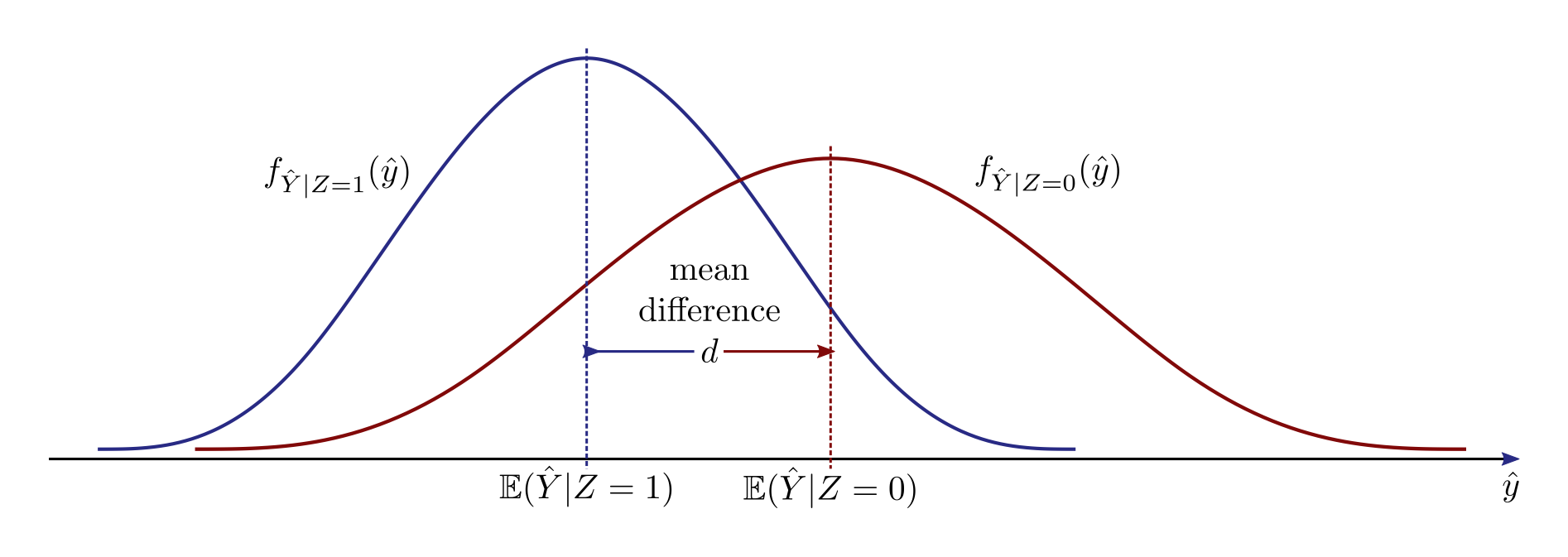
Taking the simplest example of discrete binary classifier where we have a binary sensitive feature. We can write the requirement of independence as, \[\mathbb{P}(\hat{Y}=1 | Z=1) = \mathbb{P}(\hat{Y}=1 | Z=0).\] This criterion goes by many names in research literature - demographic parity, statistical parity and parity impact, among others. We can quantify the disparity by looking at the difference or the ratio of the acceptance rates for each sensitive feature. Both are straightforward to calculate given the 2 \(\times\) 2 contingency table (Table 3.1), which summarises the observed relationship between the sensitive feature and outcome. Each cell of the contingency table shows the number of examples satisfying the conditions given in the corresponding row and column headers. So for example, \(n_{01}\) is the number of data points for which \(Z=0\) and \(\hat{Y}=1\).
| \(\hat{Y}=1\) | \(\hat{Y}=0\) | Total | |
|---|---|---|---|
| \(Z=1\) | \(n_{11}\) | \(n_{10}\) | \(n_{Z=1}\) |
| \(Z=0\) | \(n_{01}\) | \(n_{00}\) | \(n_{Z=0}\) |
| Total | \(n_{\hat{Y}=1}\) | \(n_{\hat{Y}=0}\) | \(n\) |
In bio-medical sciences, the risk difference: \[d = \mathbb{P}(\hat{Y}=1 | Z=0) - \mathbb{P}(\hat{Y}=1 | Z=1) = \frac{n_{11}}{n_{Z=0}} - \frac{n_{01}}{n_{Z=1}},\] measures the impact of treatment (or risk factors), \(Z\) on outcome, \(\hat{Y}\). In discrimination literature, it has been described as the discrimination score and statistical parity difference among others. Note that if \(\hat{Y}=1\) is the advantageous outcome and \(Z=1\) is the advantaged group, we would expect \(d\) to be negative. The algorithm is fair when \(d=0\). The further from zero, the greater the disparity. A modified version of this metric is the normalised difference[52] [52] I. Zliobaite, “On the relation between accuracy and fairness in binary classification.” 2015.Available: https://arxiv.org/abs/1505.05723 which divides the risk difference by it’s maximal value, thus ensuring the normalised difference is bounded between plus and minus one.
Statistical Parity Difference Maximum
| \[ d_{\max} = \min\left\{ \frac{\mathbb{P}(\hat{Y}=1)}{\mathbb{P}(Z=1)}, \frac{\mathbb{P}(\hat{Y}=0)}{\mathbb{P}(Z=0)} \right\} = \min\left\{ \frac{n_{\hat{Y}=1}}{n_{Z=1}}, \frac{n_{\hat{Y}=0}}{n_{Z=0}} \right\},\] | (3.5) |
Alternatively, we could instead take the ratio as a measure of discrimination: \[r = \frac{\mathbb{P}(\hat{Y}=1 | Z=0)}{\mathbb{P}(\hat{Y}=1 | Z=1)} = \frac{n_{11}/n_{Z=0}}{n_{01}/n_{Z=1}}.\] In biomedical sciences this measure is called the risk ratio. It is used to measure the strength of association between treatment (or risk factors), \(Z\), and outcome, \(\hat{Y}\). It has been described in discrimination aware machine learning literature as the impact ratio or disparate impact ratio. The algorithm is fair if \(r=1\). If we take \(Z=1\) to be the advantaged group the value is bounded between zero and one. The Equal Employment Opportunity Commission (EEOC) have used this measure in their guidelines for identifying discrimination in employment selection processes[53] [53] U. S. E. E. O. Commission, “Questions and answers to clarify and provide a common interpretation of the uniform guidelines on employee selection procedures,” Federal Register, vol. 44, no. 43, 1979. . As a rule of thumb, the EEOC determine that a company’s selection system is having an adverse impact on a particular group if the selection rate for that group is less than four-fifths (or 80%) that of the most advantaged group, that is, the impact ratio is less than 0.8 where \(Z=0\) is the most advantaged group (for which the acceptance rate is the highest).
The elift ratio[54] [54] D. Pedreschi, S. Ruggieri, and F. Turini, “Discrimination-aware data mining,” in Proceedings of the ACM SIGKDD international conference on knowledge discovery and data mining, 2008, pp. 560–568. doi: 10.1145/1401890.1401959. is similar to the impact ratio but instead of comparing acceptance rates for protected groups to each other, we compare them to the overall/mean acceptance rate: \[\frac{\mathbb{P}(\hat{Y}=1 | Z=0)}{\mathbb{P}(\hat{Y}=1)}.\]
In theory, any measure of association suitable for the data types can be used as a metric to understand the magnitude of discrimination in our data or predictions. The odds ratio (popular in natural, social and biomedical sciences) is the ratio of the odds of a positive prediction for each group. We can write it as: \[\frac{\mathbb{P}(\hat{Y}=1 | Z=1)\mathbb{P}(\hat{Y}=0 | Z=0)} {\mathbb{P}(\hat{Y}=0 | Z=1)\mathbb{P}(\hat{Y}=1 | Z=0)} = \frac{n_{11}n_{00}}{n_{10}n_{01}}.\] The odds ratio is equal to one when there is no discrimination. In the case where \(\hat{Y}=1\) in the advantaged outcome and \(Z=1\) is the privileged group, the odds ratio is always greater than or equal to one. Recall that the odds ratio is not a collapsible measure (see section 1.4.3).
As mentioned earlier, independence metrics can be evaluated on both the data and the model. A common problem in machine learning is that existing biases in the data can be exaggerated if protected groups are minorities in the population. By comparing metrics for the data with those of our model output, we can understand if our model is inadvertently introducing biases that do not originate from the data.
It might seem intuitive already, that independence can only be satisfied by a model (optimising for predictive performance), if the target variable \(Y\) and sensitive feature \(Z\) are in fact independentWe’ll prove this to be true in section 3.3, for the case where our variables are binary.
. If this is not the case, then satisfying independence for one’s model, will not permit the theoretically perfect solution \(\hat{Y}=Y\) (should your model be able to achieve it). We would also then naturally, expect that the stronger the relationship between the sensitive feature and target, the greater the trade-off with utility in satisfying independence criterion.
Independence does not guarantee fairness in a broader sense. Consider a simple hypothetical example where, there are discrepancies between credit card approval rates for men and women at the population level, which disappear once you control for (the confounding variable) income. The underlying issue appears to be the fact that women, generally earn less than men. If the lender was to enforce independence between gender and its loan approval rate by, for example, setting lower income requirements for women than men, this could conceivably lead to higher default rates among women. Clearly a less than desirable solution which, arguably, doesn’t address the underlying problem. Furthermore, it might be argued that satisfying independence could lead to less fair outcomes from a different perspective; that a man and woman who were the same in all other respects (features) would receive different outcomes. In the next chapter we’ll talk about individual fairness which reconciles these differences in perspective by requiring the specification of a task specific similarity metric for individuals.
It is important to note that the assumption of independence does not allow for confounding variables (discussed in section 1.4). Suppose we want to measure the relationship between the sensitive feature and outcome using one of the above metrics. A natural solution to the problem of confounding variables, is to control for them (assuming you have them recorded in your dataset and your data is representative of the population). Next, we consider the case where we condition on all the non-sensitive variables \(X\).
3.1.2 The Twin Test
The twin test tries to establish cause (of differing treatment across protected groups), by conditioning on all other features. Because of this, it has been interpreted as avoiding disparate treatment[49]. While legally speaking such proof is not required to establish liability (as discussed in section 1.3.2), the twin test provides a useful tool for evaluating feature specific discrimination in models. In this case, our fairness criterion requires the predicted target variable to be independent of the sensitive features when conditioned on all other features. This is true, if and only if, the probability distribution of \(Y\) conditioned on \(X\) is the same, for all values of the sensitive feature \(Z\); \[\hat{Y} \bot Z | X \quad \Leftrightarrow \quad f_{\hat{Y}|X}(\hat{y}, z; x) = f_{\hat{Y}|X}(\hat{y}; x).\]
Suppose we wish to establish a causal connection between the decision or outcome and an individual’s membership in some protected group. Typically, in a human decision process which is subjective, proving a causal connection difficult (a problem addressed by judicial systems). In the case where a decision is made purely on the basis of a deterministic algorithm (which one has access to and need only be in the form of a black box), making this causal connection is easier. Imagine a ‘counterfactual’ world in which for every individual in this world (say John Doe) there exists an identical twin in the counterfactual world which differers only by the sensitive feature (say Jane Doe). If a deterministic model produces predictions that are different for for John and Jane, we have established the individual’s sensitive feature as the reason.
With this approach, establishing cause with a model becomes straight forward. We conduct a randomized experiment, sampling for \(X\). The individuals for which we check the model output need not exist, we can simply fabricate them, and compare the target distributions. What if the model is not deterministic but rather makes randomised predictions for a given \(X\)? This makes things a bit more complicated because neither John nor Jane Doe get the same model prediction at every trial, so it’s not enough to check the outcome for a single John and Jane for each Doe. This makes the test computationally more expensive. We need to compute the target \(\hat{Y}\) a sufficiently large number of times to obtain the distribution for each value of \(X\). For a dataset, the twin test is less reliable. Without access to the (potentially human and thus non-deterministic) algorithm by which it was produced, we have no way of producing counterfactual twins that don’t exist, making sample size a potential issue.
The counterfactual approach to establishing the fairness of our model, we can consider all independence metrics described above have natural extensions which are conditioned on \(X\) as well as \(Z\). So for example we define the causal mean difference as \[\mathbb{E}(\hat{Y} | Z=1, X=x) - \mathbb{E}(\hat{Y} | Z=0, X=x).\] and the observed mean difference as \[\mathbb{E}(Y | Z=1, X=x) - \mathbb{E}(Y | Z=0, X=x).\]
3.2 Comparing Errors
In this section we learn about fairness criteria which compare model errors across groups, rather than outcomes. A fundamental assumption here is that the training data is fair and just and that there exists a ground truth to compare our model to. We discussed earlier in the chapter how independence and twin test constraints have been interpreted as avoiding disparate impact and disparate treatment respectively. Analogously, criteria on model errors have been described as avoiding disparate mistreatment[49] in the literature.
3.2.1 Independent Errors
Independence in errors (or equivalently predictive performance), is the next strongest fairness criterion after independence, \((\hat{Y}-Y) \bot Z\).
A relaxation of this criterion compares only the mean error \(\mathbb{E}(\hat{Y} - Y)\) for the groups (rather than the full distributions). This essentially tells us if essentially if our model is over or underestimating the target \(Y\) (or score \(P\) for classification) on average. For classification problems it provides a measure of the number of false positives compared to false negatives. If \(\mu\) is positive there are more false positives and vice versa. Another way to look at the mean error is a measure of luck or opportunity. Depending on whether it is preferable to have a model under or overestimate \(Y\) determines which direction is lucky (given greater opportunity) versus unlucky. For regression models Balanced residuals[55] [55] T. Calders, A. Karim, F. Kamiran, W. Ali, and X. Zhang, “Controlling attribute effect in linear regression,” 2013. doi: 10.1109/ICDM.2013.114. takes the difference of the mean errors, \[d_{\text{err}} = \mathbb{E}(\hat{Y} - Y | Z=1) - \mathbb{E}(\hat{Y} - Y | Z=0).\] This can be calculated for \(n=n_0+n_1\) data points as, \[d_{\text{err}} = \frac{1}{n_1}\sum_{i|z_i=1}(\hat{y}_i-y_i). - \frac{1}{n_0}\sum_{i|z_i=0}(\hat{y}_i-y_i)\]
For a classification problem a relaxation of this criterion compares only the error rates (or equivalently accuracy) for all groups. The direction of the error is effectively assumed to be inconsequential. To derive a measure of fairness from this criterion we could (as before) take the difference, or the ratio. The error rate difference is given by, \[\mathbb{P}(\hat{Y}\neq Y | Z=1) - \mathbb{P}(\hat{Y}\neq Y | Z=0).\] The error rate ratio is given by \[\frac{\mathbb{P}(\hat{Y}\neq Y | Z=0)}{\mathbb{P}(\hat{Y}\neq Y | Z=1)}.\] For a binary classifier, false positives and false negatives will typically have different implications and associated costs which are ignored when comparing error rates. Table 3.2 summarises terminology for the different types of error rates for a binary classification model. Table 3.3 summarises terminology for the equivalent predictive performance metrics.
| Ground Truth | ||||
|---|---|---|---|---|
| \(y=1\) | \(y=0\) | Error Rate Type | ||
| Prediction | \(\hat{y}=1\) | True Positive | False Positive Type I Error |
False Discovery Rate \(\mathbb{P}(\hat{y}\neq y|\hat{y}=1)\) |
| \(\hat{y}=0\) | False Negative Type II Error |
True Negative | False Omission Rate \(\mathbb{P}(\hat{y}\neq y|\hat{y}=0)\) |
|
| Error Rate Type | False Negative Rate \(\mathbb{P}(\hat{y}\neq y|y=1)\) |
False Positive Rate \(\mathbb{P}(\hat{y}\neq y|y=0)\) |
Error Rate \(\mathbb{P}(\hat{y}\neq y)\) |
|
| Ground Truth | ||||
|---|---|---|---|---|
| \(y=1\) | \(y=0\) | Metric | ||
| Prediction | \(\hat{y}=1\) | True Positive | False Positive Type I Error |
Positive Predictive Valuea \(\mathbb{P}(\hat{y}=y|\hat{y}=1)\) |
| \(\hat{y}=0\) | False Negative Type II Error |
True Negative | Negative Predictive Value \(\mathbb{P}(\hat{y}=y|\hat{y}=0)\) |
|
| Metric | True Positive Rateb \(\mathbb{P}(\hat{y}=y|y=1)\) |
True Negative Rate \(\mathbb{P}(\hat{y}=y|y=0)\) |
Accuracy \(\mathbb{P}(\hat{y}=y)\) |
|
a Positive Predictive Value = Precision
b True Positive Rate = Recall
Fairness criteria that compare error distributions (or equivalently predictive performance metrics) across groups can be broken down into conditional independence constraints on the joint distributions of the sensitive features, \(Z\), the target feature \(Y\) and predicted target \(\hat{Y}\). Separation conditions on \(Y\) (the columns of the confusion matrix) requiring the false negative and false positive (or equivalently the true positive and true negative) rates to be independent of protected group membership. Sufficiency conditions on \(\hat{Y}\) (the rows of the confusion matrix) requiring the false discovery and false omission (or equivalently positive predictive value and negative predictive value) rates to be independent of protected group membership. Let’s take a closer look at them.
3.2.2 Separation
Separation requires the predicted target variable to be independent of the sensitive feature, conditioned on the target variable, that is, \(\hat{Y} \bot (Z|Y)\). We can say that the predicted target \(\hat{Y}\), is separated from the sensitive feature \(Z\), by the target variable \(Y\). The corresponding graphical model for separation criteria is shown in Figure 3.2.

So, for a fixed value of the target variable, there should be no difference in the distribution of the predicted target variable, across different values of the sensitive feature. That is, \[\mathbb{P}(\hat{y}|y, z) = \mathbb{P}(\hat{y}|y).\] Unlike independence, separation, allows for dependence between the predicted target variable and the sensitive feature but only to the extent that it exists between the actual target variable and the sensitive feature.
For a binary classifier where we have a single sensitive binary feature. We can write this requirement (most well known as equalised odds[56] [56] M. Hardt, E. Price, and N. Srebro, “Equality of opportunity in supervised learning.” 2016.Available: https://arxiv.org/abs/1610.02413 ) as two conditions, \[\begin{aligned} \mathbb{P}(\hat{Y}=1 | Z=1, Y=1) & = \mathbb{P}(\hat{Y}=1 | Z=0, Y=1), \\ \mathbb{P}(\hat{Y}=1 | Z=1, Y=0) & = \mathbb{P}(\hat{Y}=1 | Z=0, Y=0). \end{aligned}\] Recall that \(\mathbb{P}(\hat{Y}=1 | Y=1)\) is the true positive rate (\(TPR\)) of the classifier and \(\mathbb{P}(\hat{Y}=1 | Y=0)\) is the false positive rate (\(FPR\)). We see then that separation requires the true positive rate, and the false positive rate, to be the same for all values of the sensitive feature.
Let’s think about what this means in the context of a recidivism risk predictor used in sentencing. Separation requires the proportion of (false positive) errors among those that did not in fact reoffend, and (false negative) errors among those that did to be the same across protected groups. This was essentially Propublica’s criticism of COMPAS, that the model overestimated the risk presented by Black defendants (demonstrated by their higher false positive rate) and underestimated the risk presented by White defendants (demonstrated by their higher false negative rate).
Two related metrics are the average odds difference and average odds error. The average odds difference measures the magnitude of unfairness as the average of the difference in true positive rate and false positive rate, \[\frac{1}{2} [ TPR_{Z=0} - TPR_{Z=1} + FPR_{Z=0} - FPR_{Z=1} ].\] The average odds error measures the magnitude of unfairness as the average of the absolute difference in true positive rate and false positive rate, \[\frac{1}{2} [ |TPR_{Z=0} - TPR_{Z=1}| + |FPR_{Z=0} - FPR_{Z=1}| ].\]
A relaxed version of equalised odds, called equal opportunity[56], requires only the true positive rates to be the same across all groups, assuming a positive prediction is the advantageous or lucky outcomeRecall Rawl’s second principle of justice as fairness (fair equality of opportunity) discussed in section 1.2.
. If the reverse is true (i.e. the negative prediction is the advantageous outcome), we would instead want the true negative rates to be equal. For our recidivism risk predictor, this would mean ensuring that for defendants which did not reoffend have the same probability of being flagged low risk. Said another way, we want defendants that were in fact low risk to be given equal opportunity to be marked low risk across protected groups. A metric which uses this as a criterion to measure unfairness is equal opportunity difference which takes the difference in true positive rates across groups, that is, \[TPR_{Z=0} - TPR_{Z=1}.\]
3.2.3 Sufficiency
Sufficiency requires the sensitive feature \(Z\) and target variable \(Y\) to be independent, conditional on the predicted target variable \(\hat{Y}\), that is, \(Y \bot (Z|\hat{Y})\). We can say that the predicted target \(\hat{Y}\) is sufficient for the sensitive feature \(Z\). That is to say, given \(\hat{Y}\), \(Z\) provides no additional information. The corresponding graphical model for sufficiency criteria is shown in Figure 3.3.

It should hopefully be straightforward to see that sufficiency requires the false omission rate and false discovery rate (see Table 3.2) to be equal across protected groups.
Sufficiency
Sufficiency is satisfied if and only if the false omission rate and false discovery rate are equal for all groups. Proof in appendix D.1.
Sufficiency requires the probability of of an error for a given prediction to be the same across protected groups. Let’s think about what this means for our binary recidivism risk calculator. Sufficiency requires that for a given prediction (high/low risk), the probability of error (predicting high risk for those that did not reoffend/predicting low risk for those that did) is independent of protected group membership.
Comparing sufficiency to separation we note that \(Y\) and \(\hat{Y}\) are reversed in the graphical models (and conditional independence constraints). In the graphical model for separation, the data is upstream of the model output; for sufficiency, we assume the model is upstream of the data. In reality of course, the world is more complicated. In the previous chapter we discussed the machine learning cycle - specifically the fact that including a model in the decision making process impacts future data, which, when used to retrain our model, creates feedback loops. In imposing both separation and sufficiency (by requiring independent errors), we accept that our causal model is more complicated - like that shown in Figure 3.4 a).
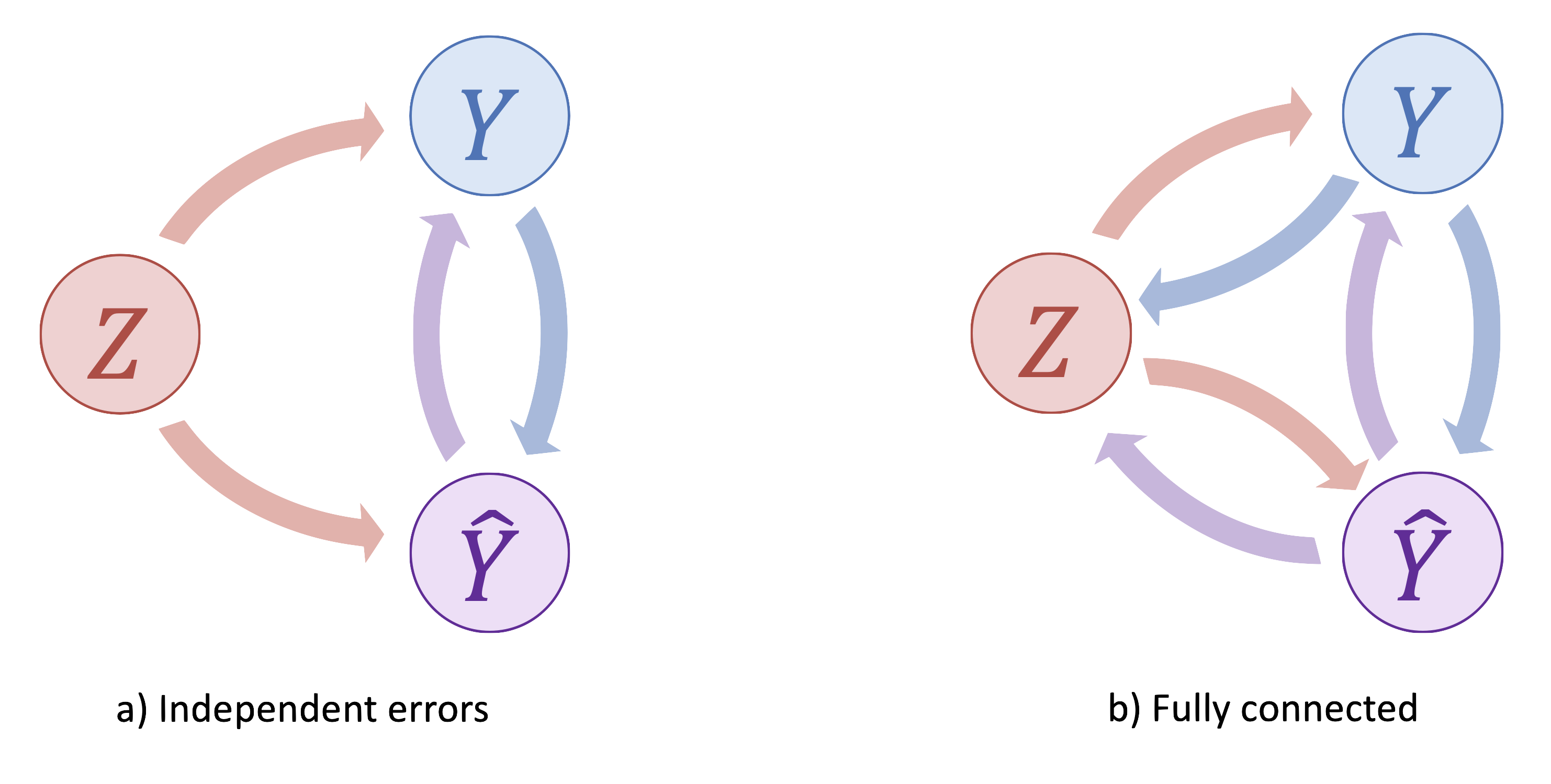
We tend to think of sensitive features as immutable facts, but in reality they are not. Over time, we can expect a progressive society to become more inclusive, recognising more subgroups that previously did not exist. If we accept that environmental factors, and even our target or prediction, can affect the sensitive categories we fall into, the graph then perhaps begins to look more like Figure 3.4 b), at which point, there’s little value to be found in graphical models, because everything is connected. But it’s worth realising just how much more complicated reality typically is, especially when decisions that can shape lives are at stake.
Sufficiency and Calibration by Group
As one might expect, satisfying separation or sufficiency does not require as great a sacrifice of utility as independence (assuming \(Y\not\perp Z\)). Neither separation nor sufficiency are necessarily satisfied by the utility optimal solution. Of the two sufficiency, imposes a weaker constraint on our model. To understand why, we explore another interpretation of sufficiency which intuitively explains why it might be satisfied implicitly through the training process[57]
[57] L. T. Liu, M. Simchowitz, and M. Hardt, “The implicit fairness criterion of unconstrained learning.” 2019.Available: https://arxiv.org/abs/1808.10013
. Let us look at sufficiency criteria in terms of the classification score \(P\), \[\mathbb{P}(Y=1 | P=p, Z=1) = \mathbb{P}(Y=1 | P=p, Z=0) \quad \forall \, p\] We say that a classifier score is calibrated if \[\mathbb{P}(Y=1 | P=p) = p \quad \forall \, p.\] Essentially, this is the requirement that the proportion of data points assigned the score \(p\), which did in fact have a positive outcome \(Y=1\), should be equal to the score \(p\). The score \(p\) can then be interpreted, at the population level, as the probability that the a positive prediction \(\hat{Y}=1\) would be correctFor the score to be interpretable as this probability at the individual level, we would need to satisfy the stronger criteria \(P=\mathbb{E}[Y|X]\).
.
From the definitions above we can see that if our classifier scores are calibrated for all groups, sufficiency is automatically satisfied. If our model satisfies sufficiency but not calibration by group, we can calibrate our model score through a simple transformation. We simply pick a value for \(Z\), \(Z=1\) say, and then calculate the mapping, \[\mathbb{P}(Y=1|P=p, Z=1) = f(p).\] We then transform all our scores to new scores (which satisfy calibration by group) by applying the inverse mapping \(f^{-1}(P)\). The resulting model is both sufficient and calibrated. It’s worth noting that the developers of COMPAS were able to demonstrate that their model did satisfy calibration by group. In a later review, researchers crowd sourced human risk assessors via Amazon Mechanical Turk it was found that COMPAS was "no more accurate or fair than predictions made by people with little or no criminal justice expertise. In addition, despite COMPAS’s collection of 137 features, the same accuracy can be achieved with a simple linear classifier with only two features"[58] [58] J. Dressel and H. Farid, “The accuracy, fairness, and limits of predicting recidivism,” Science Advances, vol. 4, no. 1, p. eaao5580, 2018, doi: 10.1126/sciadv.aao5580. .
There are some obvious advantages of comparing errors rather than outcomes. Note that unlike criteria comparing outcomes they do not preclude the theoretically perfect solution, \(\hat{Y}=Y\). The criteria also preclude large differences in error rates for different groups that are typical when disadvantaged classes are minorities suffering from low support. It’s worth reiterating that criteria comparing errors assume that the relationship between \(Y\) and \(Z\) prescribed by the training data is fair. Depending on the context of the problem one might prioritise equalising one type of error over another. For example, in pretrial risk assessment we might choose to prioritise ensuring equal false positive rates if we believe that it is preferable to set free a guilty defendant than incarcerate an innocent one. As another example, let’s take the infamous NYPD stop-and-frisk program where pedestrians were stopped, interrogated and searched on ‘reasonable’ suspicion of carrying contraband. In this case we might want to ensure false discovery rates are equal across groups to ensure we are not disproportionately targeting particular minority groups.
3.3 Incompatibility Between Fairness Criteria
So far in this chapter we have learned a range of different group fairness criteria and seen how each of them can be viewed as imposing different constraints on the joint distributions of our variables \(X\), \(Z\), \(Y\) and \(\hat{Y}\). In this section we will prove that these fairness criteria can be restrictive enough to mean that satisfying more than one of them is impossible, except in some degenerate cases. For a useful recap of the rules of probability (which we will use in our proofs), see in Appendix C.
3.3.1 Independence versus Sufficiency
Independence versus Sufficiency
Independence (\(Z \bot \hat{Y}\)) and sufficiency (\(Z \bot Y | \hat{Y}\)) can only be simultaneously satisfied if the sensitive feature, \(Z\) and the target variable \(Y\) are independent (\(Z \bot Y\)).
To prove this we consider the conditional distribution \(Z|Y,\hat{Y}\).
| \[\begin{aligned} \textrm{Independence: } Z \bot \hat{Y} \quad & \Rightarrow\quad \mathbb{P}(z|y,\hat{y}) = \mathbb{P}(z|y) \nonumber\\ \textrm{Product rule} \quad & \Rightarrow\quad \mathbb{P}(z|y) = \frac{\mathbb{P}(z,y)}{\mathbb{P}(y)}\nonumber\\ & \Rightarrow\quad \mathbb{P}(z|y,\hat{y}) = \frac{\mathbb{P}(z,y)}{\mathbb{P}(y)}. \end{aligned}\] | (3.6) |
Applying Sufficiency, followed by independence gives,
| \[\begin{aligned} \textrm{Sufficiency: } Z \bot Y | \hat{Y} \quad & \Rightarrow\quad \mathbb{P}(z|y,\hat{y}) = \mathbb{P}(z|\hat{y})\nonumber\\ \textrm{Independence: } Z \bot \hat{Y} \quad & \Rightarrow\quad \mathbb{P}(z|\hat{y}) = \mathbb{P}(z)\nonumber\\ & \Rightarrow\quad \mathbb{P}(z|y,\hat{y}) = \mathbb{P}(z). \end{aligned}\] | (3.7) |
Equating (3.6) and (3.7) and rearranging gives, \[\mathbb{P}(z,y) = \mathbb{P}(z)\mathbb{P}(y).\] Thus, \(Z\) and \(Y\) must be independent.
3.3.2 Independence versus Separation
Independence versus Separation
In the case that \(Y\) is binary, independence (\(Z \bot \hat{Y}\)) and separation (\(Z \bot \hat{Y} | Y\)) criteria can only be simultaneously satisfied if either \(\hat{Y} \bot Y\) or \(Y \bot Z\).
To prove this we consider the distribution of \(\hat{Y}\).
| \[\begin{aligned} \textrm{Sum rule:} \quad & \Rightarrow \quad \mathbb{P}(\hat{y}) = \sum_{y\in\mathcal{Y}} \mathbb{P}(\hat{y}, y).\nonumber\\ \textrm{Product rule} \quad & \Rightarrow \quad \mathbb{P}(\hat{y}) = \sum_{y\in\mathcal{Y}} \mathbb{P}(\hat{y}|y) \mathbb{P}(y). \end{aligned}\] | (3.8) |
| \[\begin{aligned} \textrm{Conditioning on }Z \quad \Rightarrow \quad \mathbb{P}(\hat{y}|z) = \sum_{y\in\mathcal{Y}} \mathbb{P}(\hat{y}|y, z) \mathbb{P}(y|z).\nonumber\\ \textrm{Independence: } \hat{Y} \bot Z \quad \Rightarrow \quad \mathbb{P}(\hat{y}) = \sum_{y\in\mathcal{Y}} \mathbb{P}(\hat{y}|y) \mathbb{P}(y|z). \end{aligned}\] | (3.9) |
Equating (3.8) and (3.9) and rearranging gives,
| \[ \sum_{y\in\mathcal{Y}} \mathbb{P}(\hat{y}|y) [\mathbb{P}(y)-\mathbb{P}(y|z)] = 0\] | (3.10) |
For binary \(Y\), \(\mathcal{Y}=\{0,1\}\). Denoting \(\mathbb{P}(y)=p_y\) and \(\mathbb{P}(y|z) = q_y\), then \(p_1 = 1-p_0\) and \(q_1 = 1-q_0\). Substituting into (3.10) gives, \[\begin{aligned} & \phantom{[}\mathbb{P}(\hat{y}|Y=0)(p_0-q_0)+\mathbb{P}(\hat{y}|Y=1)[1-p_0-(1-q_0)] = 0 \\ \Leftrightarrow \quad & [\mathbb{P}(\hat{y}|Y=0)-\mathbb{P}(\hat{y}|Y=1)](p_0-q_0) = 0 \end{aligned}\] which is true if and only if, \[\begin{aligned} &\textrm{either } & \mathbb{P}(\hat{y}|Y=0) = \mathbb{P}(\hat{y}|Y=1) \quad & \Leftrightarrow \quad \hat{Y} \bot Y,\\ & \textrm{or } & p_0=q_0 \quad \Leftrightarrow \quad \mathbb{P}(Y=0) = \mathbb{P}(Y=0|z) \quad & \Leftrightarrow \quad Y \bot Z. \end{aligned}\]
3.3.3 Separation versus Sufficiency
Separation versus Sufficiency I
In the case where all events in the joint distribution of \(Z\), \(Y\) and \(\hat{Y}\) have non zero probability, separation (\(Z \bot \hat{Y} | Y\)) and sufficiency (\(Z \bot Y | \hat{Y}\)) can only be simultaneously be satisfied if the sensitive feature, \(Z\) is independent of both the target variable \(Y\) and the predicted target \(\hat{Y}\), that is if \(Z \bot Y\) and \(Z \bot \hat{Y}\).
To prove this we consider the conditional distribution \(\mathbb{P}(z|y,\hat{y})\).
| \[\begin{aligned} \textrm{Separation: } Z \bot \hat{Y} | Y \quad & \Rightarrow \quad \mathbb{P}(z|y,\hat{y}) = \mathbb{P}(z|y) \nonumber\\ \textrm{Sufficiency: } Z \bot Y | \hat{Y} \quad & \Rightarrow \quad \mathbb{P}(z|y,\hat{y}) = \mathbb{P}(z|\hat{y}) \nonumber\\ & \Rightarrow \quad \mathbb{P}(z|y) = \mathbb{P}(z|\hat{y}). \end{aligned}\] | (3.11) |
| \[\begin{aligned} \textrm{Product rule: } \quad\phantom{\Rightarrow} \mathbb{P}(z,y) & = \mathbb{P}(z|y) \mathbb{P}(y)\nonumber\\ (3.11) \qquad\quad \Rightarrow \quad \mathbb{P}(z,y) & = \mathbb{P}(z|\hat{y}) \mathbb{P}(y). \end{aligned}\] | (3.12) |
\[\begin{aligned} \textrm{Sum rule: } \quad \phantom{\Rightarrow}\mathbb{P}(z) & = \sum_{y\in\mathcal{Y}} \mathbb{P}(z,y)\\ (3.12) \quad\,\, \Rightarrow \quad \mathbb{P}(z) & = \sum_{y\in\mathcal{Y}} \mathbb{P}(z|\hat{y}) \mathbb{P}(y) \end{aligned}\] If all events have non-zero probability, we can move \(\mathbb{P}(z|\hat{y})\) outside of the summation,
| \[ \mathbb{P}(z) = \mathbb{P}(z|\hat{y})\] | (3.13) |
Thus showing that \(Z\) and \(\hat{Y}\) must be independent. Equating (3.11) and (3.13) shows that \(Z\) and \(Y\) must also be independent.
Separation versus Sufficiency II
In the case where \(Y\) is binary, separation and sufficiency can only be satisfied simultaneously if the sensitive feature is independent of the target variable, or the model has an accuracy of 100% (\(\hat{Y}=Y\)) or 0% (\(\hat{Y}=1-Y\)).
Consider the case where \(Y\) is binary. Separation requires all groups to have the same true positive rate (recall or \(TPR\)) and the same false positive rate (\(FPR\)). On the other hand, sufficiency requires all groups to have the same positive predictive value (precision or \(PPV\)) and the same negative predictive value (\(NPV\)). A problem is evident at this point. For a fixed number of data points, the confusion matrix for a binary classifier only has three degrees of freedom but satisfying both separation and sufficiency introduces four constraints which requires four degrees of freedom in order be able to satisfy them. We can write the positive and negative predictive values in terms of the true positive and false positive rates.
Predictive Values
We can write the positive and negative predictive values in terms of the true and false positive rates as follows,
| \[ PPV = \frac{p TPR}{p TPR + (1-p)FPR}\] | (3.14) |
and
| \[ NPV = \frac{(1-p)(1-FPR)}{p(1-TPR) + (1-p)(1-FPR)}\] | (3.15) |
For separation to hold the true positive rate (\(TPR\)) and false positive rate (\(FPR\)) must be constant across all values of the sensitive features. For sufficiency to hold the positive predictive value (\(PPV\)) and negative predictive value (\(NPV\)) must be constant across all values of the sensitive features. For brevity we shall denote \(p_a=\mathbb{P}(Y=1|Z=a)\).
Separation versus Sufficiency
For separation and sufficiency to hold we must have
| \[ FPR (p_a-p_b) TPR = 0\] | (3.16) |
and
| \[ (1-FPR) (p_a-p_b) (1-TPR) = 0\] | (3.17) |
for any pair of groups \(Z=a\) and \(Z=b\). Proof in appendix D.1.
Equations (3.16) and (3.17) can only be simultaneously satisfied in 3 cases:
\(p_a=p_b \, \forall \, a, b\) in which case \(Y \bot Z\),
\(FPR=0\) and \(TPR=1\) in which case \(Y=\hat{Y}\),
\(FPR=1\) and \(TPR=0\) in which case \(Y=1-\hat{Y}\).
3.4 Concluding Remarks
We’ve seen that in general, for a binary classifier, there are only a few cases in which it is possible to satisfy more than one of the three group fairness criterion simultaneously. It’s a useful exercise to summarise our findings, because this will provide some clues as to how we might go about improving our model/s of fairness. Table 3.4 provides such a summary.
| Comparing | Name | Criterion | ||||
|---|---|---|---|---|---|---|
| Strong | \(\displaystyle \hat{Y}\bot Z\quad \left\{ \rule[-3.3em]{0pt}{7em} \right.\) | Outcomes | Independence | \(\displaystyle \hat{Y}\bot Z\) | \(\displaystyle \left.\rule[-1.3em]{0pt}{2.8em} \right\}\quad\hat{Y}\bot Y\) or \(\displaystyle |Y|>|Z|\) | |
| \(\displaystyle \Bigg\uparrow\) | Errors | Separation | \(\displaystyle \hat{Y}\bot Z|Y\) | \(\displaystyle \left.\rule[-2.5em]{0pt}{5.4em} \right\}\) | ||
| \(\displaystyle \hat{Y}=Y\) or \(\displaystyle \hat{Y} = 1-Y\) | ||||||
| Weak | Errors | Sufficiency | \(\displaystyle Y\bot Z|\hat{Y}\) |
There are two types of fairness metrics, those comparing outcomes or predictions \(\hat{Y}\), and those comparing errors. We can further bisect the latter into separation and sufficiency. The criteria are ordered from strong to weak; by this we are referring to the trade-off with utility in satisfying it. Independence or statistical parity is the strongest criterion. There is a larger gap between separation and sufficiency, because separation imposes a more similar constraint to independence. We still want the sensitive feature to be independent of the prediction, but only when conditioned on the actual outcome \(Y\). Sufficiency is almost implicitly satisfied just by training or calibrating our model. All three criteria compare some joint distribution over the prediction, target and sensitive feature. The brackets either side of the table show which sets of criteria can be satisfied and how.
Independence and sufficiency (at the top and bottom of Table 3.4 respectively) are the furthest apart; they can only be satisfied if the actual outcome \(Y\) is independent of \(Z\). This says that all sensitive subgroups must be equally represented in both the accepted and rejected groups in the data. But if \(Y\) is independent of \(Z\), we can satisfy all three criteria. It makes sense that the gold standard for fairness is representation, because fairness is aspirational.
Separation and sufficiency are the next closest together. If we could only satisfy two of the three criteria, these are the ones we’d choose, because together they give us independent errors. This is only possible, if the target and prediction are exactly the same, or exactly the opposite; that is, if the error is always exactly zero, or exactly one. This makes sense, because independent errors, does not prohibit the target \(Y\) or prediction \(\hat{Y}\) from depending on \(Z\). Rather, it’s okay for them to depend on \(Z\), as long as their difference doesn’t. For a binary target, there are only two ways of satisfying this constraint.
Lastly, we can satisfy independence and separation if the prediction \(\hat{Y}\) is independent of the target (which sounds like a terrible model) or if the target \(Y\) has more degrees of freedom than \(Z\). So for a binary sensitive feature, we need three or more possible outcomes, to satisfy both independence and separation. Note that if we have infinitely possible outcomes, as in the case of a continuous target, we can definitely satisfy both these criteria, because \(Z\) is certainly finite in size (limited to a finite number of subgroups). Furthermore, if the target is continuous, that would help us to satisfy independence of errors, without requiring equal representation. So increasing the degrees of freedom in our target seems like a promising path.
There is one particular issue with group fairness metrics. That is, that equalising statistical properties at the group level, does not guarantee fair treatment at an individual level. Let’s return to our applicant filter with the sensitive feature gender. Independence requires that acceptance rates are equal for male and female applicants. Suppose model acceptance rates are lower for female applicants. To ensure we satisfy the independence fairness criterion, we could just randomly select female applicants that were rejected and instead accept them until the acceptance rates matched. In fact this kind of approach can be used to satisfy any group fairness criterion. Clearly this method will likely result in some undeserving female applicants being accepted. Although this approach would be able to satisfy the fairness criterion, the resulting algorithm would likely be considered unfair.
It’s worth noting that although the approach of randomly selecting female applicants to accept might seem unnecessarily naive, there can be cases, (particularly when there are multiple protected characteristics that intersect) where protected groups are so small that models simply do not have enough training data to be able to make accurate predictions for them. In such cases a model could conceivably be, not much better than guessing for individuals in those groups. Even if we supposedly take a smarter approach of say, choosing the individuals closest to the decision boundary (rather than choosing them randomly) this would be equivalent to choosing a different acceptance threshold for women, in which case we would be using a different criterion to determine acceptance for male and female applicants (which are in all other respects similar), which could be viewed as unfair, despite satisfying independence. In the next chapter we’ll talk about individual fairness which resolves these difficulties by specifying the modelling problem in such a way that the notions of fairness and utility are entirely orthogonal.
Summary
Group fairness
The term group fairness is used to describe a class of metrics that are used to measure discrimination or bias across specific subgroups of a population, in a given decision process. At the implementation level, all group fairness metrics indicate the extent to which, some statistical property differs between different groups.
In general group fairness criterion and measures can be derived from independence constraints on the joint distributions of the non-sensitive features \(X\), sensitive features, \(Z\), the target feature \(Y\) and predicted target \(\hat{Y}\).
Group fairness criteria can be broadly classified into two types; those that compare outcomes and those comparing errors.
| Comparing | Outcomes | Errors | ||
|---|---|---|---|---|
| Criterion | Independence | Twin Test | Separation | Sufficiency |
| Constraint | \(\hat{Y}\bot Z\) | \(\hat{Y}\bot Z|X\) | \(\hat{Y}\bot Z|Y\) | \(Y\bot Z|\hat{Y}\) |
| Measures | Disparate impact | Disparate treatment | Disparate mistreatment | |
Comparing Outcomes
| Category | Criterion | Definition |
|---|---|---|
| Independence \(\hat{Y}\bot Z\) |
Mutual information | \(\displaystyle I(\hat{Y},Z)=\sum_{z\in\mathcal{Z}}\,\,\int_{\hat{y} \in \mathcal{Y}} f_{\hat{Y},Z}(\hat{y},z) \log \frac{f_{\hat{Y},Z}(\hat{y},z)} {f_{\hat{Y}}(\hat{y})\mathbb{P}(z)}\,\mathrm{d}\hat{y}\) |
| Normalised prejudice index | \(\displaystyle r_{\text{npi}} = \frac{I(\hat{Y},Z)}{\sqrt{S(\hat{Y})S(Z)}}, \quad S(Z) = -\sum_{z\in\mathcal{Z}} \mathbb{P}(z)\log\mathbb{P}(z)\) | |
| Mean difference | \(\displaystyle d = \mathbb{E}(\hat{Y} | Z=0) - \mathbb{E}(\hat{Y} | Z=1)\) | |
| Statistical paritya | \(\displaystyle \mathbb{P}(\hat{Y}=1 | Z=1) = \mathbb{P}(\hat{Y}=1 | Z=0)\) | |
| Risk differenceb | \(\displaystyle d = \mathbb{P}(\hat{Y}=1 | Z=0) - \mathbb{P}(\hat{Y}=1 | Z=1)\) | |
| Normalised difference | \(\displaystyle \bar{d} = \frac{d}{d_{\max}}, \quad d_{\max} = \min\left\{ \frac{\mathbb{P}(\hat{Y}=1)}{\mathbb{P}(Z=1)}, \frac{\mathbb{P}(\hat{Y}=0)}{\mathbb{P}(Z=0)} \right\}\) | |
| Risk ratioc | \(\displaystyle r = \frac{\mathbb{P}(\hat{Y}=1 | Z=0)}{\mathbb{P}(\hat{Y}=1 | Z=1)}\) | |
| Elift ratio | \(\displaystyle \frac{\mathbb{P}(\hat{Y}=1 | Z=0)}{\mathbb{P}(\hat{Y}=1)}\) | |
| Odds ratio | \(\displaystyle \frac{\mathbb{P}(\hat{Y}=1 | Z=1)\mathbb{P}(\hat{Y}=0 | Z=0)} {\mathbb{P}(\hat{Y}=0 | Z=1)\mathbb{P}(\hat{Y}=1 | Z=0)}\) | |
| Twin test \(\hat{Y}\bot Z|X\) |
Causal mean difference | \(\displaystyle \mathbb{E}(\hat{Y} | Z=1, X=x) - \mathbb{E}(\hat{Y} | Z=0, X=x)\) |
| Observed mean difference | \(\displaystyle \mathbb{E}(Y | Z=1, X=x) - \mathbb{E}(Y | Z=0, X=x)\) |
aAlso called, demographic parity and parity impact.
bAlso called, discrimination score and statistical parity difference.
cAlso called, impact ratio and disparate impact ratio.
Independence (\(\hat{Y}\bot Z\))
Independence metrics can be evaluated on both data and model output. Comparing them is important in understanding if our model is inadvertently introducing or exaggerating biases in the training data.
If the target variable \(Y\) and sensitive feature \(Z\) are not independent then imposing it on a model does not permit the theoretically perfect solution \(Y = \hat{Y}\). The stronger the relationship between \(Z\) and \(Y\), the greater the trade-off between fairness and utility in satisfying independence criterion.
Independence does not consider the existence of confounding variables.
In the case where independence is not satisfied by the data, imposing it on a model implies a level of distrust in the data or modelling of the problem.
The Twin Test (\(\hat{Y}\bot Z|X\))
The twin test tries to establish cause (of differing treatment across protected groups), by comparing results for counterfactual twins that differ only by group membership.
Given access to the model in the form of a black box, the twin test consists of a randomised experiment, sampling individuals and comparing the output for the corresponding twins.
For a stochastic model, the twin test is computationally more expensive, since we must evaluate our model for each pair of twins a sufficiently large number of times to obtain the predicted target distribution.
Comparing errors
Criteria comparing errors assume that the data is fair.
Unlike criteria comparing outcomes, criteria comparing errors do not preclude the theoretically perfect solution, \(\hat{Y}=Y\).
| Category | Criterion | Definition |
|---|---|---|
| Error \((\hat{Y}-Y)\bot Z\) |
Balanced residuals | \(d_{\text{err}} = \mathbb{E}(\hat{Y} - Y | Z=1) - \mathbb{E}(\hat{Y} - Y | Z=0)\) |
| Error rate | Error rate difference | \(\mathbb{P}(\hat{Y}\neq Y | Z=1) - \mathbb{P}(\hat{Y}\neq Y | Z=0)\) |
| Error rate ratio | \(\displaystyle \frac{\mathbb{P}(\hat{Y}\neq Y | Z=0)}{\mathbb{P}(\hat{Y}\neq Y | Z=1)}\) | |
| Separation \(\hat{Y}\bot Z|Y\) |
Equalised odds | \(TPR_{Z=0} = TPR_{Z=1}\) and \(TNR_{Z=0} = TNR_{Z=1}\) |
| Average odds difference | \(\frac{1}{2} [ TPR_{Z=0} - TPR_{Z=1} + FPR_{Z=0} - FPR_{Z=1} ]\) | |
| Average odds error | \(\frac{1}{2} [ |TPR_{Z=0} - TPR_{Z=1}| + |FPR_{Z=0} - FPR_{Z=1}| ]\) | |
| Equal opportunity | \(TPR_{Z=0} = TPR_{Z=1}\) | |
| Equal opportunity difference | \(TPR_{Z=0} - TPR_{Z=1}\) | |
| Sufficiency \(Y\bot Z|\hat{Y}\) |
Equally sufficient | \(PPV_{Z=0} = PPV_{Z=1}\) and \(NPV_{Z=0} = NPV_{Z=1}\) |
| Calibration by group | \(\mathbb{P}(Y=1 | P=p, Z=z) = p \quad \forall \, p, z\) |
Separation (\(\hat{Y}\bot Z|Y\))
Separation, allows for dependence between the predicted target variable and the sensitive feature but only to the extent that it exists between the actual target variable and the sensitive feature.
Sufficiency (\(Y\bot Z|\hat{Y}\))
For a binary classification model, sufficiency requires the probability of of an error for a given prediction to be equal across protected groups.
A model that is calibrated by group satisfies sufficiency.
Sufficiency is is a weaker model constraint compared to separation as it is satisfied implicitly through the training process.
Incompatibility between fairness criteria
Independence (\(Z \bot \hat{Y}\)) and sufficiency (\(Z \bot Y | \hat{Y}\)) can only be simultaneously be satisfied if the sensitive feature \(Z\), and the target variable \(\hat{Y}\), are independent (\(Z \bot Y\)).
In the case that \(Y\) is binary, independence (\(Z \bot \hat{Y}\)) and separation (\(Z \bot \hat{Y} | Y\)) criteria can only be simultaneously satisfied if either \(\hat{Y} \bot Y\) or \(Y \bot Z\).
Separation (\(Z \bot \hat{Y} | Y\)) and sufficiency (\(Z \bot Y | \hat{Y}\)) can only be simultaneously be satisfied if the sensitive feature, \(Z\) is independent of both the target variable \(Y\) and the predicted target \(\hat{Y}\), that is if \(Z \bot Y\) and \(Z \bot \hat{Y}\).
In the case where \(Y\) is binary, separation and sufficiency can only be satisfied simultaneously if the sensitive feature is independent of the target variable, or the model has an accuracy of 100% (\(\hat{Y}=Y\)) or the model has an accuracy of 0% (\(\hat{Y}=1-Y\)).
Concluding remarks
We need more degrees of freedom in the target variable. Would ensure we are always able to satisfy independent errors.
Equalising statistical properties at the group level, don’t guarantee fair treatment at an individual level.
4 Individual Fairness
This chapter at a glance
Fairness at an individual level
Individual fairness as continuity
Individual fairness as uncertainty
Individual fairness as consistency
Broadly speaking, individual fairness is the idea that a given decision process is fair, if similar people (with respect to the task), receive similar decisions. Compared to group fairness, individual fairness is arguably a much more expansive concept of fairness. Group fairness criteria are rather specific. They tackle the question of fairness by comparing pairs of groups but this approach has limitations. In particular, equalising statistical properties at the group level, don’t guarantee fair treatment for any given individual. What do we mean by fairness at an individual level and how does it relate to group fairness? Let’s go back to our applicant filter. We wanted to understand if our algorithm is biased against female applicants. What if there are more than two genders? Then we need to calculate our metric on all the subgroups. But what we really want to do is make sure we’re being fair to all intersections of protected features too - disadvantages (and indeed advantages) on multiple dimensions can compound. As we create finer grained partitions of the population, we increase the number of groups. Eventually every group contains a single individual. In order to measure fairness at an individual level then, we need a way of comparing individuals rather than groups - a similarity metric.
As a measure, individual fairness cares not about the decision itself, but rather about the consistency with which decisions are made. Individual fairness is a property of a mapping from features to output (\(Y\) or \(\hat{Y}\)), not a measure of how one mapping differs from another (\(\hat{Y}-Y\)). In this sense, utility and individual fairness are orthogonal. It’s not immediately obvious but this is an important conceptual leap from group fairness but it is. Individual fairness does not assume the existence of a fair ground truth dataset in its definition of fairness; it cares only how similar people are, (not how to rank them, that is the job of utility function). The similarity metric represents the ground truth for what is fair; that is, how similar people are (with respect to the task) in feature space.
In this chapter we’ll provide the formal definition of individual fairness (as originally proposed by Dwork et. al.[59] [59] C. Dwork, M. Hardt, T. Pitassi, O. Reingold, and R. Zemel, “Fairness through awareness.” 2011.Available: https://arxiv.org/abs/1104.3913 ). We will see that by this notion of fairness, deterministic classification models are inherently unfair. We resolve this issue by returning a distribution over outcomes and sampling predictions randomly from our distribution. Finally, we look at popular measures of individual fairness and analyse them. Let’s get started!
4.1 Individual Fairness as Continuity
What does individual fairness mean for a model? Let’s start with a deterministic regression model and think of it as a function that maps individuals to predictions. Individual fairness can then be interpreted as a requirement that, two points that are close in input (feature) space are also close in output (target/prediction) space. To satisfy this constraint our model mapping must be continuous. At a discontinuity, two individuals falling either side of it can be arbitrarily similar (identical) in feature space and yet receive entirely different outcomes. Below we define Lipschitz ContinuityNamed after the German mathematician Rudolf Lipschitz, perhaps most well known for his contributions to mathematical analysis.
in the context of a deterministic regression model.
Lipschitz Continuity (Regression)
Consider \(\hat{y}\), to be determined by our model function \(f\) which maps individuals \(\boldsymbol{x}\in\mathcal{X}\) to predictions \(\hat{y}\in\mathcal{Y}\), that is to say \(\hat{y}=f(\boldsymbol{x})\) and \(f:\mathcal{X}\mapsto\mathcal{Y}\). The function \(f\) is Lipschitz continuous if there exists a real valued, non-negative constant \(K\in\mathbb{R}_{\geq 0}\) such that, for every pair of individuals \(\boldsymbol{x}_i, \boldsymbol{x}_j \in \mathcal{X}\),
| \[ d_{\mathcal{Y}}(f(\boldsymbol{x}_i), f(\boldsymbol{x}_j)) \leq K d_{\mathcal{X}}(\boldsymbol{x}_i, \boldsymbol{x}_j).\] | (4.1) |
Where \(d_{\mathcal{X}}:\mathcal{X}\times\mathcal{X}\mapsto\mathbb{R}\) and \(d_{\mathcal{Y}}:\mathcal{Y}\times\mathcal{Y}\mapsto\mathbb{R}\) are distance metrics (the properties of which we recap below) that allow us to determine how close (similar) any two points are in the feature and target spaces respectively. \(K\) is called the Lipshitz constant.
For the simplest case where all our features and the target are real values, that is \(\mathcal{X}=\mathbb{R}^m\) and \(\mathcal{Y}=\mathbb{R}\), our model \(\hat{y}=f(\boldsymbol{x})\), can be visualised as an \(m+1\) dimensional surface. In this case, we can interpret continuity as the requirement that the slope of our model (with respect to our similarity metric) is finite and bounded between \(\pm K\) on the domain \(\mathcal{X}\). The smaller the slope, the more similarly neighbouring individuals are treated. We can apply this idea to a finite set of data points, \(\mathcal{X}=\{\boldsymbol{x}_1,\boldsymbol{x}_2,...,\boldsymbol{x}_n,\}\) and \(\mathcal{Y}=\{y_1, y_2,...,y_n\}\), (again where \(\boldsymbol{x}_i\in\mathbb{R}^m\,\forall\, i\) and \(y_i\in\mathbb{R}\)). If the gradient of the line between any two data points in the dataset is bounded between \(\pm K\) then there no evidence that the mapping violates the criterion.
Distance metric properties
A distance metric \(d\) on the set \(\mathcal{X}\) is a function \(d:\mathcal{X}\times\mathcal{X}\mapsto\mathbb{R}_{\geq 0}\) that has the following properties \(\forall\,\,x, y, z\in\mathcal{X}\)
Identity: \(d(x,y)=0 \Leftrightarrow x=y\)
Symmetry: \(d(x,y)=d(y,x)\)
Triangle inequality: \(d(x,y)\leq d(x,z)+d(z,y)\)
Combining Symmetry with the triangle inequality shows that the metric must return a non-negative value.

4.2 Individual Fairness as Randomness
For classification problems our target variable is discrete, the example falls into one class or another and we treat individuals differently based on their classification. Our job applicant filter either accepts or rejects an applicant, there isn’t anything in between. Then how can a classification model satisfy continuity and thus individual fairness? It can’t. A deterministic classifier indeed cannot satisfy individual fairness by construction because it has a discontinuity at the decision boundary. For example, let’s suppose our job applicant filter outputs a score. We use a threshold \(t=0.5\) on the score, so we accept the applicant if their score is greater than or equal to 0.5 and reject them if they score lower. At a score of 0.5 the probability of acceptance ‘jumps’ from zero to one. The threshold \(t=0.5\) defines the decision boundary. We will reject an applicant that scores 0.4999 but accept an applicant that scores 0.5 despite them being the same (within error say) according to our model. See Figure 4.2.
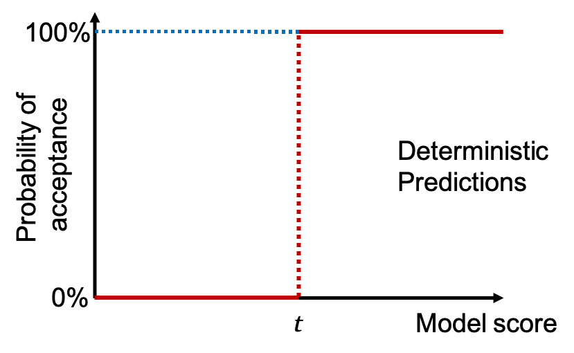
If we want our model to be fair at the individual level, we need to remove the discontinuity (close the gap) at our decision boundary. How might we do this? Let’s return to our simple example of the job applicant filter. Let’s assume our binary classifier outputs a score and that score is a continuous function of our features. In this case, the discontinuity in our model mapping is a result of the threshold alone because continuity holds under composition. That is to say, a continuous function of a continuous function is also continuousMore precisely, for \(f(x)=g(h(x))\), if \(h(x)\) is continuous at \(x=a\) and \(g(x)\) is continuous at \(x=h(a)\) then \(f\) is continuous at \(x=a\).
. Then if we can remove the discontinuity at the threshold our model mapping will be continuous. Rather than imposing a threshold on the model score and rejecting or accepting individuals based on which side of the threshold they fall, we can use the score to determine the probability of acceptance. We then randomly draw a value according to that probability distribution, to determine if the individual is accepted or not. This approach allows the probability of acceptance to be a continuous function of model score. See for example Figure 4.3.
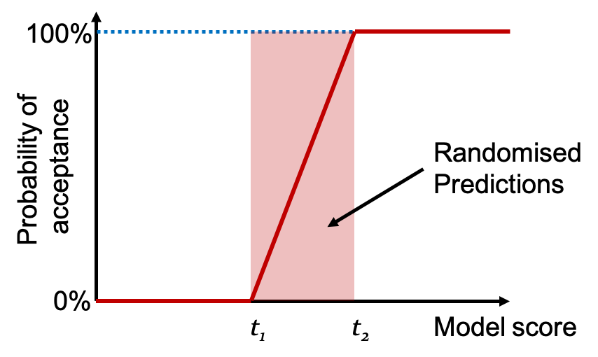
At first glance, this approach might sound bizarre. We are saying that in order to remedy the problem that similar individuals receive different predictions, we must instead turn to a model which can make different predictions for the same individual?! Indeed the definition of consistency in judgement is a debated topic among legal scholars. For some randomness is explicitly forbidden[60] [60] A. V. Dicey, “The law of the constitution.” 1978. , others allow flexibility in the interpretation of the rules[61] [61] R. Dworkin, “No right answer.” 1978. but not randomness in the decision. Clearly there is value in being able to make a single and predictable judgement most of the time. That might mean favouring one decision over another in the face of uncertainty. But the value of certainty is in itself is contextual. In legal decisions, the stakes are high, we need a process for making the decision that provides some confidence that we are correct and so we might favour letting a guilty person go free than an innocent person be incarcerated (beyond reasonable doubt so to speak) but this need not always be the case.
With a deterministic model we allow arbitrarily similar individuals to be guaranteed to receive different predictions. By randomising our predictions we accept that in any decision, we may have incomplete or erroneous knowledge (and thus uncertainty in our predictions). At the very least there is uncertainty around the decision boundary where individuals (according to our own model) fall into the maybe category. For those individuals, the decision is more a matter of luck (or risk depending on your perspective) than others. By moving to a stochastic model we are able to always gives similar individuals a similar chance of being accepted (or rejected). Randomness in predictions in machine translation for example makes complete sense. If the translation of a word in a sentence has 55% probability of being the masculine variation and 40% chance of being the feminine variation (according to your own model) then does it always make sense to consistently predict the masculine? In this example we see more clearly how randomness in predictions when faced with uncertainty can be desirable trait when it comes to being fair. In Figure 4.3 we illustrate the simplest way to achieve continuity at the decision boundary. We create a region (between two thresholds \(t_1\) and \(t_2\)) in which model scores result in randomised predictions. Implementation in appendix D.2.
For classification then, our model must be probabilistic, that is, it maps each individual in feature space to a distribution over the possible outcomes, which we can then randomly draw from to make predictions. Our predictions are then randomised rather than deterministic and to satisfy individual fairness we require our probabilistic model mapping to be continuous. Let’s write our continuity condition for our classifier more formally.
Lipschitz Continuity (Classification)
Consider our classification model to be a function \(f\), which maps individuals \(\boldsymbol{x}\in\mathcal{X}\) and outcomes \(y\in\mathcal{Y}\) to probabilities \(p_{\boldsymbol{x}}(y)\), that is to say \(p_{\boldsymbol{x}}(y)=f(\boldsymbol{x}, y)\) and \(f:\mathcal{X}\times\mathcal{Y}\mapsto[0,1]\). For a fixed value of \(\boldsymbol{x}\), \(p_{\boldsymbol{x}}(y)=f(\boldsymbol{x}, y) \in \mathcal{P}(\mathcal{Y})\) is a distribution over all possible outcomes \(y\in\mathcal{Y}\). Then the mapping \(f\) is Lipschitz continuous if there exists a real valued, non-negative constant \(K \in \mathbb{R}_{\geq 0}\) such that,
| \[ d_{\mathcal{P}(\mathcal{Y})}(f(\boldsymbol{x}_i,y), f(\boldsymbol{x}_j,y)) \leq K d_{\mathcal{X}}(\boldsymbol{x}_i, \boldsymbol{x}_j) \quad \forall\,\, \boldsymbol{x}_i, \boldsymbol{x}_j \in \mathcal{X}\] | (4.2) |
where \(d_{\mathcal{X}}:\mathcal{X}\times\mathcal{X}\mapsto\mathbb{R}\) and \(d_{\mathcal{P}(\mathcal{Y})}:\mathcal{P}(\mathcal{Y})\times\mathcal{P}(\mathcal{Y})\mapsto\mathbb{R}\) denote distance metrics. \(d_{\mathcal{X}}\) determines how similar two individuals are in feature space and \(d_{\mathcal{P}(\mathcal{Y})}\) measures how similar two probability distributions over \(\mathcal{Y}\) are.
We now have a theoretical understanding of how individual fairness translates to a model behaviour, ideally our model mapping is continuous and the smaller the slope of the surface (with respect to our similarity metric), the more similarly neighbouring individuals are treated. In fact, if the slope is zero everywhere then everyone is treated the same. All individuals get mapped to the same distribution over outcomes and we have satisfied our individual fairness constraint. Of course such a model would not make a very good predictor as it would not take into account the features of the individuals in its predictions. We can then think of the problem of satisfying individual fairness as an additional constraint in our model optimisation task. We want to maximise utility (minimise some loss function \(\mathcal{L}\), on the training data) and to satisfy individual fairness we want to ensure the slope of our model, with respect to our similarity metric is bounded between \(\pm K\). In practice we can absorb the value \(K\) into our similarity metric \(d_{\mathcal{X}}(\boldsymbol{x}_i, \boldsymbol{x}_j)\). Notice that we are indifferent to the direction of the slope, we care only about its size. Getting the direction of the slope right is achieved by maximising utility. Thus we have reduced our problem of training a fair model to one of constrained optimisation. \[\begin{aligned} & \min\left\{\mathbb{E}_{\boldsymbol{x}\in\boldsymbol{X}}\, \mathbb{E}_{\hat{Y}\sim f(\boldsymbol{x},Y)}\,\left[\mathcal{L}(\boldsymbol{X}, \boldsymbol{Y}, \boldsymbol{\hat{Y}})\right]\right\}, \\ \textrm{such that}\quad & d_{\mathcal{P}(\mathcal{Y})}(f(\boldsymbol{x}_i,y), f(\boldsymbol{x}_j,y)) \leq d_{\mathcal{X}}(\boldsymbol{x}_i, \boldsymbol{x}_j) \\ \textrm{and}\quad & \quad f(\boldsymbol{x_i},y) \in \mathcal{P}(\mathcal{Y})\qquad\forall\,\boldsymbol{x}_i, \boldsymbol{x}_j \in \boldsymbol{X}. \end{aligned}\]
4.3 Similarity Metrics
4.3.1 Similarity Between Individuals
A question we have glossed over so far is on the similarity metrics \(d_{\mathcal{X}}(\boldsymbol{x}_i, \boldsymbol{x}_j)\). It might not seem like we have gained much in reframing fairness as treating similar people similarly. After all, we still have to specify a similarity metric. Determining how similar individuals (or more generally examples in feature space) are, is a question that we answer either explicitly or implicitly by machine learning solutions when maximising utility. In practice the requirement of defining a similarity metric exposes our definition of fairness and decouples it from utility (or predictive performance). Recall in the last chapter, when considering different notions group fairness we saw different trade-offs with utility. Individual fairness unifies these different definitions of fairness by exposing our belief about what is fair (be it anti classification, anti-subordination or something in between) in the form of a similarity metric. In some sense it provides a better model for fairness. A particular advantage of this framework is that it allows separation of the classification task between two distinct parties, a data owner and a model user. The data owner is a trusted party while the model user is the party who wishes to classify individuals. Under the proposed constrained optimisation framework, the model user is free to define the loss function, but the classification task (map from individuals to distributions over outcomes) could be the responsibility of the trusted data owner.
4.3.2 Similarity Between Probability Distributions
Let’s look at two possible choices for \(d_{\mathcal{P}(\mathcal{Y})}\).
Total Variation (\(L_1\)) Norm: \(D_{1}\)
One possible distance metric on distributions \(d_{\mathcal{P}(\mathcal{Y})}\) is the total variation, \[d_{\mathcal{P}(\mathcal{Y})} = d_{tv}(p,q) = \frac{1}{2} \sum_{y\in\mathcal{Y}} |p(y)-q(y)|.\] Note that \(d_{tv}\) is bounded between zero (when the distributions are the same) and one (when the distributions are entirely non-overlapping), therefore the Lipschitz condition would require us to the choose the distance metric \(d_{\mathcal{X}}\) between individuals to be scaled similarly. This can be problematic depending on the feature space.
Relative (\(L_{\infty}\)) Norm: \(D_{\infty}\)
An alternative choice for \(d_{\mathcal{P}(\mathcal{Y})}\) which resolves this issue is the relative \(l_{\infty}\) metric: \[d_{\mathcal{P}(\mathcal{Y})} = d_{\infty}(p,q) = \sup_{y\in\mathcal{Y}} \log \left[\max\left(\frac{p(y)}{q(y)}, \frac{q(y)}{p(y)}\right)\right].\]
4.4 Measuring Individual Fairness in Practice
The metric consistency, measures individual fairness by looking at the changes in our model output for neighbouring points on a finite set of data points. \[yNN = 1 - \frac{1}{n} \sum_{i=1}^n \left| \hat{y}_i - \frac{1}{k}\sum_{j|x_j\in kNN(\boldsymbol{x}_i)} \hat{y}_j \right|\] It is described as measuring “the consistency of the model classifications locally in input space”[62] [62] R. Zemel, Y. Wu, K. Swersky, T. Pitassi, and C. Dwork, “Learning fair representations,” in Proceedings of the 30th international conference on machine learning, 2013, vol. 28, pp. 325–333. . Values close to one indicate that similar inputs are treated similarly. Note that if all individuals receive the same prediction, consistency will be exactly one. The consistency metric described above, rather conveniently, avoids the need to choose a metric that compares probability distributions over outcomes but we still need a distance metric in feature space to compare how similar two individuals are and thus find the \(k\) nearest neighbours.
Summary
Individual fairness is the idea that a given decision process is fair, if similar people (with respect to the task) receive similar decisions. As a measure, individual fairness cares not about the actual decision, but rather about the consistency with which they are made.
Individual fairness is orthogonal to utility, it does not factor a ground truth \(\hat{Y}\) into it’s calculation, it is only interested in the change in prediction relative to the similarity. That is a property of a mapping.
Individual fairness can be interpreted as a continuity requirement on our data or model. In practice it can be implemented by imposing a bound on the slope of our model mapping, with respect to our similarity metric.
A deterministic classifier (one that typically outputs a score and then imposes a threshold on it to determine the predicted class) cannot satisfy individual fairness by construction, because the threshold results in a discontinuity in the model mapping where the gradient becomes infinite.
For a classification model to satisfy individual fairness (continuity) we must turn to a probabilistic model which maps individuals to distributions over outcomes. The continuity requirement then applies to the change in distribution of outcomes relative to the similarity of individuals. Predictions must be randomised, based on the model output distributions.
The metric consistency is given by \[yNN = 1 - \frac{1}{n} \sum_{i=1}^n \left| \hat{y}_i - \frac{1}{k}\sum_{j|x_j\in kNN(\boldsymbol{x}_i)} \hat{y}_j \right|.\] It uses \(k\)-Nearest Neighbours to measure the consistency of model classifications locally in input space in an effort to quantify individual fairness in a dataset. Values close to one indicate that similar inputs are treated similarly.
5 Utility as Fairness
This chapter at a glance
Inequality indices for ranking distributions.
Subgroup decomposability of generalised entropy indices
A unified approach to measuring fairness across individuals and groups
Minimising inequality as maximising utility
Analysing the behaviour of the index as a function of model performance metrics
In this chapter we review inequality indices and their application in measuring algorithmic fairness. More specifically, “measuring how unequally the outcomes of an algorithm, benefit different individuals or groups in a population”[63] [63] T. Speicher et al., “A unified approach to quantifying algorithmic unfairness,” Proceedings of the 24th ACM SIGKDD International Conference on Knowledge Discovery & Data Mining, 2018, doi: 10.1145/3219819.3220046. . Inequality indices measure divergence from the uniform distribution and as such are an important tool for measuring fairness. They are used extensively in economics and social development to measure inequality in metrics across individuals and groups in a population. Indices such as the coefficient of variation, Gini and Theil are well known tools for measuring income inequality. Their application extends beyond fairness to any problem where there is value in understanding how far from uniformly distributed a given attribute is, for example measuring racial segregation and the efficiency of distributed systems.
Let’s dive in with an overview of the proposed application to predictive algorithms. Using inequality indices to measure algorithmic unfairness is a two step process. First, we must define a benefit function which maps the outcome of an algorithm to the corresponding benefit. Next, given the resulting benefits for a group of individuals, we can calculate the value of the index for that group, by simply plugging the values into the formula for the index. The value of the index provides a measure of how unfair the algorithm is, in its distribution of benefits over that group. The larger the value of the index or inequality measure, the more unequally, the benefits are distributed. There are then two fundamental questions we must answer in measuring algorithmic unfairness in this way.
Index calculation: There are lots of measures available that each rank inequality in different ways, which one should we use?
Benefit function: How do we map our predictions to benefits?
Inspired by the work of Speicher, Heidari et al.[63] (here on in referred to as the original paper), we discuss these questions, specifically for algorithmic classifiers. Following their work, we focus our attention on generalised entropy indices, a special family of inequality indices that are subgroup decomposable, into a between-group component and within-group component. We show how generalised entropy indices can be viewed as the class of subgroup decomposable loss functions. We analyse the effect of the generalisation parameter \(\alpha\) and show that for \(\alpha=0\), the index is a linear function of the cross entropy loss. We show that in the special case \(\alpha=1/2\), the contribution to the total loss from the between-group component is maximised. For the benefit function proposed in the original paper, which we describe as equal luck, we provide an analytical account of the index’s behaviour as a function of the generalisation parameter \(\alpha\), model accuracy \(\lambda\), and mean error \(\mu\).
5.1 Measuring Inequality
Let’s start by deriving perhaps the most well known inequality index, the Gini index (named after statistician Corrado Gini). To do this we need to introduce some notation. We denote the benefits received by each individual, in our population size \(n\), as the vector \(b=(b_1, b_2,...,b_n)\). For convenience we assume the benefit vector, \(\boldsymbol{b}\) is sorted in ascending order. If the benefits are sorted, it’s straight forward to calculate the cumulative income distribution, that is the total income earned by the bottom \(p\) percent of the population. Since we are not interested in the actual amounts individuals earn, but rather how much they earn relative to each other, we rescale to construct the Lorenz curve \(F(p)\) (named after the economist Max Lorenz). The Lorenz curve is a piecewise linear function which tells us the percentage of total income earned by the bottom \(p\) percent. Figure 5.1 shows an example Lorenz curve.
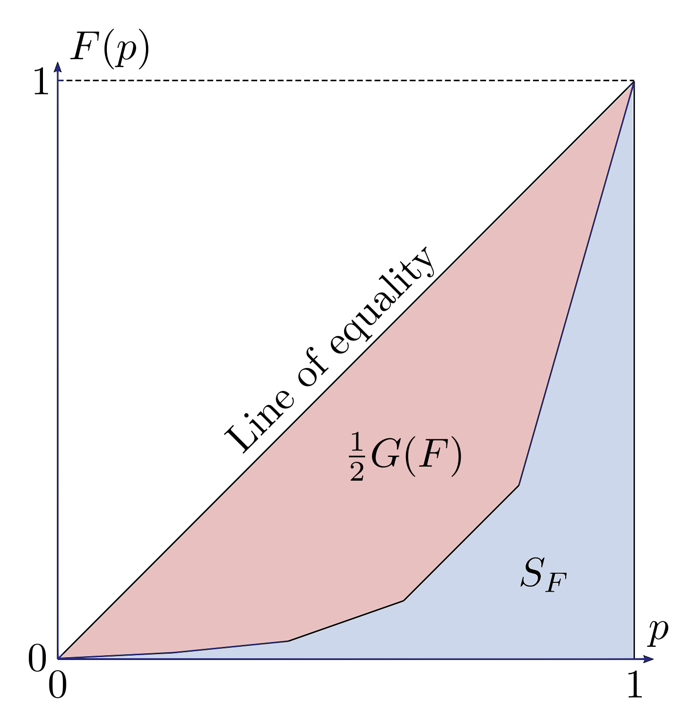
The Lorenz curve has some interesting properties by construction. We know that \(F(0)=0\) and \(F(1)=1\). The curve is always increasing and convex, that is increasing at an increasing rate. This means, the first and second derivatives are always positive. It should be intuitive that the smaller the area under the Lorenz curve \(S_F\), the greater the inequality. The area between the line of equality and \(F(p)\) then provides a measure of inequality and doubling it means it has a maximal value of one and minimal value of zero (or more accurately \(1/n\)). The Gini index is, given by \(G(F)=1-2S_F\).
Let us denote the total, mean and proportion of total benefit as, \[S_b = \sum_{i=1}^n b_i, \qquad \mu = \frac{S_b}{n} \qquad\textrm{and}\qquad p_i = \frac{b_i}{n\mu},\] respectively. Then we can write the Lorenz curve as \[F(p) = F\left(\frac{x}{n}\right) = \frac{1}{n} \sum_{i=1}^x p_i.\] We can use trapezium rule to calculate the area \(S_F\) exactly, \[S_F = \frac{1}{n} \sum_{x=1}^n \left[F\left(\frac{x}{n}\right)-\frac{1}{2}\right] = \frac{1}{n} \sum_{i=1}^n \left(n-i+\frac{1}{2}\right)p_i.\] Finally, the Gini index is given by, \[G(F) = 1 - 2S_F = \frac{2}{n} \sum_{i=1}^n (i-n)p_i = \frac{2}{n} \sum_{i=1}^n \left(\frac{i}{n}-1\right)\frac{b_i}{\mu}.\] We note that the contribution to the Gini index from any individual benefit is multiplied by its ranking.
Properties of Inequality Indices
Before getting into the particular family of indices we’ll focus on in this chapter, we mention some more general properties of inequality indices that describe their behaviour. We denote our inequality measure with \(I\) where \(I:\mathbb{R}^n_{\geq 0}\mapsto\mathbb{R}_{\geq 0}\); that is, the inequality measure maps a vector of \(n\) non-negative, real valued benefits \(\boldsymbol{b}\) to a positive real number \(I(\boldsymbol{b})\geq0\).
Anonymity / Symmetry
The inequality measure is a function of \(\boldsymbol{b}\) alone, no other characteristics of the individuals are relevant. The index is symmetric in the individual benefits. It does not matter who earned which benefit and neither does the order of the benefits \(b_i\) in the benefit vector \(\boldsymbol{b}\).
Scale invariance
The value of the index does not change under a constant scaling of the benefits. That is, for any constant \(c>0\), \(I(c\boldsymbol{b})=I(\boldsymbol{b})\).
Transfer principle
Transferring benefit, from a higher benefit individual to a lower benefit individual, must decrease the value of the measure, provided the amount of benefit transferred, does not exceed the amount required for the individuals to switch places in their benefit ranking. That is, for any \(1\leq i<j\leq n\) and \(0<\delta<(b_j-b_i)/2\), we must have \[I(b_1,...,b_i+\delta,...,b_j-\delta,....,b_n) < I(\boldsymbol{b}).\]
Zero-normalisation
The measure achieves the minimal value of zero, when all individuals receive the same benefit, \(b_i=\mu\;\forall\;i\). That is, for any \(b>0\), \(I(\mu,\mu,...,\mu)=0\)
5.2 Generalised Entropy Indices
In our analysis, we consider the one parameter family of inequality metrics known as generalised entropy indices. These represent the (entire) class of inequality measures that are additively decomposable[64] [64] A. F. Shorrocks, “The class of additively decomposable inequality measures,” Econometrica: Journal of the Econometric Society, vol. 48, no. 613–625, 1980. . This means that for any given partition of a population into distinct subgroups, generalised entropy indices can be decomposed as, the sum of a between-group (or intergroup) component, and a within-group (or intragroup) component.
Between-group component
The between-group component is computed as the value of the index, assuming all individuals receive the mean benefit, of the partition to which they belong. Essentially, it measures the contribution to the inequality index, from differences in the average benefit between the subgroups (akin to the notion of group fairness we discussed in chapter 3, except here, the relative sizes of the subgroups matter). If all the groups have the same mean benefit the between-group component is zero.
Within-group component
The within-group component is computed as a weighted sum of the index value for each subgroup, and can be thought of as measuring the contribution to overall (individual) unfairness, arising from variation in benefits between individuals in the subgroups. For a within-group component to be zero, we require every individual in the subgroup to have exactly the same benefit.
The ability to additively decompose these inequality measures into intergroup and intragroup components, is arguably where their value lies. The group fairness measures in chapter 3, make pairwise comparisons of groups. Thanks to their property of additive decomposability, generalised entropy indices have the advantage of providing a principled way of aggregating the fairness measures over any number of subgroups of the population. Historically, much of the research and development of techniques for reducing algorithmic bias, has focussed on improving group fairness metrics. Generalised entropy indices then, provide a simple way to see when trade-offs between the different notions of fairness (between-group and within-group) might occur.
Properties of Generalised Entropy Indices
Let’s summarise the more specific properties of generalised entropy indices which make them of particular interest for measuring unfairness.
Subgroup decomposability
For any partition \(G\) of the population into (mutually exclusive) subgroups, the measure \(I(\boldsymbol{b})\) can be written as the sum of a between-group component \(I_{\beta}^G(\boldsymbol{b})\) (calculated as the value of the index where all individuals are assigned the mean benefit of their subgroup) and a within-group component \(I_{\omega}^G(\boldsymbol{b})\) (calculated as a weighted sum of the index values for the subgroups).
Population invariance
The measure does not depend on the size of the population. More specifically, the value of the inequality measure does not change if we increase the population under consideration by replicating it \(k\) times. That is, if \(\boldsymbol{b}' = \langle\boldsymbol{b}, \boldsymbol{b},...,\boldsymbol{b}\rangle \in\mathbb{R}^{kn}_{\geq 0}\) is a \(k\)-replication of \(\boldsymbol{b}\), then \(I(\boldsymbol{b}')=I(\boldsymbol{b})\). Note that generalised entropy indices are the only differentiable family of inequality indices, which satisfy both population and scale invariance.
5.2.1 Index Calculation
Generalised Entropy Indices
The generalised entropy index for benefits \(b_1, b_2,...,b_n\) with mean benefit \(\mu\) can be written as
| \[ I_{\alpha}(\boldsymbol{b}) = \frac{1}{n}\sum_{i=1}^n f_{\alpha}(x_i) \quad\textrm{where}\quad x_i = \frac{b_i}{\mu}.\] | (5.1) |
\(x_i\) denotes what proportion of the mean benefit, individual \(i\) received. \(\alpha\) is a free parameter that determines the strength of the contribution to the index, from different parts of the benefit distribution.
| \[ f_{\alpha}(x) = \left\{ \begin{array}{cl} -\ln x & \textrm{if}\quad \alpha=0 \\ x\ln x & \textrm{if}\quad \alpha=1 \\ \rule{0em}{3.5ex} \dfrac{x^{\alpha}-1}{\alpha(\alpha-1)} & \textrm{if}\quad \alpha\in\mathbb{R}. \end{array}\right.\] | (5.2) |
Observation 1.
For \(\alpha\leq0\) the index is undefined for zero benefits (since \(f_{\alpha}(x)\rightarrow\infty\) as \(x\rightarrow0\)), making it unsuitable for measuring inequality where zero benefits are possible.
Given an array of benefits we can calculate what proportion of the total benefit each individual received by dividing their benefit by the sum of the benefits in the array. If the total benefit is equally divided among the population, each individual receives the mean benefit \(\mu\). If we divide the benefits by the mean benefit (rather than the sum), we calculate \(x_i=b_i/\mu\) which tells us how many times the fair (mean) amount each individual received. Notice that,
| \[ \boldsymbol{x} = \frac{\boldsymbol{b}}{\mu} = n\boldsymbol{p} \qquad\Rightarrow\qquad \boldsymbol{b} = n\mu \boldsymbol{p}\] | (5.3) |
where \(p_i\) is the proportion of the total benefit ascribed to individual \(i\). Since the index is scale invariant we know that \(I_{\alpha}(\boldsymbol{b})=I_{\alpha}(\boldsymbol{p})\). Since \(p_i\in[0,1]\;\forall\; i\), we know that \(x\in[0,n]\).
Observation 2.
Let \(B\) and \(P\) denote the random variables that generate \(b_i\) and \(p_i\) respectively. We know that \(\mathbb{E}(B)=\mu\) and \(\mathbb{E}(P)=1/n\). The generalised entropy index can be written as,
| \[ I_{\alpha}(\boldsymbol{b}) = \mathbb{E}\left[f_{\alpha}(B/\mu)\right] \qquad\textrm{or}\qquad I_{\alpha}(\boldsymbol{p}) = \mathbb{E}\left[f_{\alpha}(nP)\right]\] | (5.4) |
We know that inequality indices measure divergence from the uniform distribution and we can think of them as a system for ranking distributions from most to least fair. The most fair (and least uncertain) distribution, where everyone receives the mean benefit, has an index value of zero. In this case the benefit distribution has all of its weight at the mean \(\mu\). We can write the distribution of benefits in this case as \(\delta(b-\mu)\) where \(\delta\) is the delta function (see appendix A). To understand the role of the generalisation parameter in ranking, consider two closely related distributions with the same mean, illustrated in Figure 5.2. The first distribution \(f(b)\) is skewed, and the second is its reflection in the mean \(f(\mu-b)\).
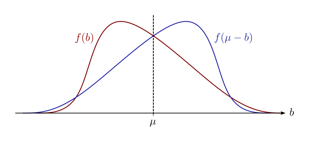
Which distribution of benefits is preferred? The generalisation parameter \(\alpha\) determines the weight \(f_{\alpha}(b/\mu)\) applied to different parts of the distribution in calculating its ranking.
5.2.2 Special Cases
Let’s review some familiar special cases of the parameter \(\alpha\) starting with zero. Suppose we have a classification model which tells us the distribution over outcomes predicted by our model, \(\boldsymbol{\hat{y}}(\boldsymbol{x}_i)\) for any individual with features \(\boldsymbol{x}_i\). Suppose that we also have the true outcome, a \(\boldsymbol{y}\) on a sample of \(n\) individuals together with. Let \(b_i=\mathbb{P}(\hat{y}_i=y_i)\) denote the probability of observing the true outcome, \(y_i\) for individual \(i\) according to our model. The cross entropy loss is given by \[\mathcal{L}(\boldsymbol{\hat{y}},\boldsymbol{y}) = \mathcal{L}(\boldsymbol{b}) = -\sum_{i=1}^n \ln(b_i).\] The cross-entropy loss is minimised at a value of zero, when all probabilities are unity. The loss is unbounded above, \(\mathcal{L}(\boldsymbol{p})\rightarrow\infty\) as \(b_i\rightarrow0\) . Notice all probabilities must be greater than zero for the integrand to be defined.
\(I_0\) and Cross Entropy Loss
| \[ \mathcal{L}(\boldsymbol{b}) = n[I_0(\boldsymbol{b})-\ln(\mu)]\] | (5.5) |
Entropy is calculated as follows, \[\mathrm{entropy}(\boldsymbol{p}) = -\sum_{i=1}^n p_i\ln(p_i),\] where \(p_i\) is the probability of the \(i\)th possible event. One interpretation of entropy is as a measure of uncertainty which is inversely related to equality. The most uncertain distribution is the most equal, the uniform distribution. It assigns every possible outcome, the same probability. The least uncertain distribution is most unequal, the delta distribution, where one outcome occurs with probability one, and all others have zero probability. For a uniform distribution with \(n\) possible events, each event occurs with probability of \(\frac{1}{n}\), in which case entropy has a maximal value of \[\max_{\boldsymbol{p}}\{\mathrm{entropy}\} = \ln(n).\] For the delta distribution, the entropy is minimal with a value of zero. For \(\alpha=1\), the generalised entropy index, is also known as the Theil index.
\(I_1\) and Entropy
| \[ I_1(\boldsymbol{b}) = I_1(n\mu\boldsymbol{p}) = \max_{\boldsymbol{p}}\{\mathrm{entropy}\} - \mathrm{entropy}(\boldsymbol{p}).\] | (5.6) |
Gini impurity (not to be confused the Gini index) is given by, \[\mathrm{Gini}(\boldsymbol{p}) = 1 - \sum_{i=1}^n p_i^2.\] It calculates the probability of misclassification if our predictions are sampled from \(\boldsymbol{p}\).
\(I_2\) and Gini Impurity
| \[ \frac{2}{n} \left[ I_2(\boldsymbol{b}) + n^2\right] = 1 - \mathrm{Gini}(\boldsymbol{p})\] | (5.7) |
In the special case \(\alpha=2\), the generalised entropy index is a monotonic increasing function of the relative standard deviation (the standard deviation divided by the mean, also known as the coefficient of variation).
\(I_2\) and Relative Standard Deviation
| \[ \frac{\sigma}{\mu} = \sqrt{2I_2(\boldsymbol{b})}.\] | (5.8) |
The standard deviation \(\sigma\) tells us how spread out (around the mean) the distribution of benefits is. So for \(\alpha=2\), the index is a monotonic increasing function of the spread and a monotonic decreasing function of the mean benefit.
The Atkinson index, which can be written as \[A_{\epsilon} = 1 - \frac{1}{\mu} \left(\frac{1}{n}\sum_{i=1}^n b_i^{1-\epsilon}\right)^{1/(1-\epsilon)},\] is related to the generalised entropy index as follows.
\(I_{\alpha}\) and the Atkinson Index \(A_{\epsilon}\)
| \[ 1 + \alpha(\alpha-1)I_{\alpha}(\boldsymbol{b}) = \left[ 1 - A_{\epsilon}(\boldsymbol{b})\right]^{\alpha}\] | (5.9) |
where \(\epsilon=1-\alpha\geq0\).
5.2.3 Behaviour with Respect to Generalisation Parameter \(\alpha\)
We can think of \(f_{\alpha}(b/\mu)\) is as a measure of the contribution to the collective disadvantage which arises from an individual with a benefit of \(b\), in a population where the mean benefit is \(\mu\). This is much like how we calculate the cost when training a model. When we fitting a model to data however, we don’t care what the total (or equivalently mean) cost is, we just want to find the model parameters that minimise it. We can think of this as fixing the value \(\mu=1\).
Observation 3.
From equation (5.2) we can show that, \[f_{\alpha}'(x) = \left\{ \begin{array}{cl} -1/x & \textrm{if}\quad \alpha=0 \\ 1+\ln x & \textrm{if}\quad \alpha=1 \\ x^{\alpha-1}/(\alpha-1) & \textrm{if}\quad \alpha\in\mathbb{R} \end{array}\right\} \qquad\textrm{and}\qquad f_{\alpha}''(x) = x^{\alpha-2}.\] Note that since \(x>0, \;f''_{\alpha}(x)>0\;\forall\;\alpha\), thus \(f_{\alpha}(x)\) is convex for all values of \(\alpha\). When \(\alpha=1\), the contribution to the inequality index is proportional to the individual benefit.
Behaviour of \(f_{\alpha}(x)\)
For \(\alpha<1\), \(f_{\alpha}(x)\) is a strictly decreasing.
For \(\alpha=1\), \(f_{\alpha}(x)\) is minimal at \(x=e^{-1}\).
For \(\alpha>1\), \(f_{\alpha}(x)\) is a strictly increasing.
In Figure 5.3, we plot the function \(f_{\alpha}(x)\), for different choices of \(\alpha\).
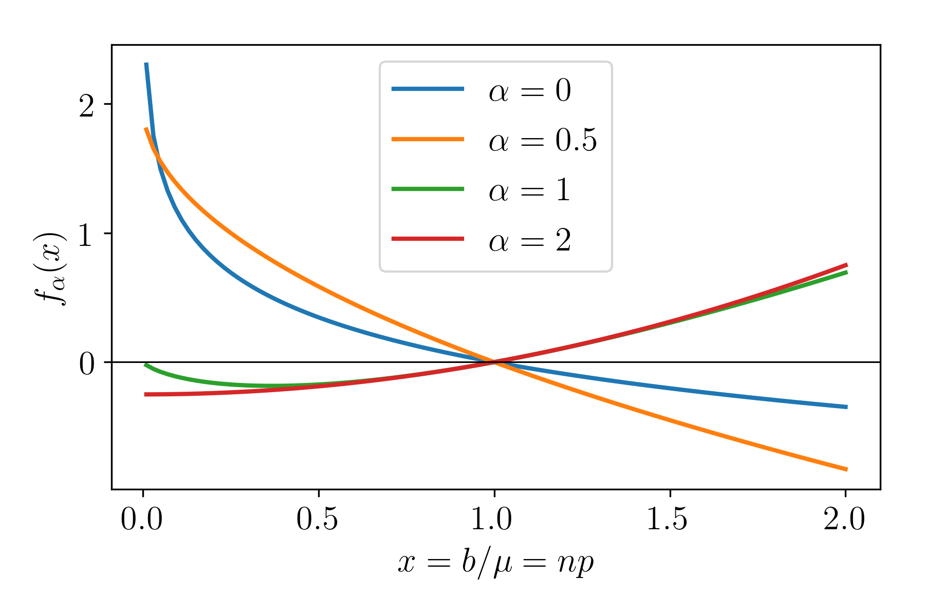
We note that the contribution to the index, from individuals that receive the mean benefit, is always zero. As we increase \(\alpha\), the contribution to the index from the upper end of the benefit distribution grows, while the contribution from the lower end decays.
For \(\alpha<1\):
A fixed transfer in benefit (from rich to poor) at the low end of the distribution (where \(f_{\alpha}(x)\) is steeply declining), decreases the the value of the index more than at the top end (where \(f_{\alpha}(x)\) is flatter).
For \(\alpha>1\):
The reverse is true. A fixed transfer in benefit (from rich to poor) at the upper end of the distribution (where the \(f_{\alpha}(x)\) is steeply increasing), decreases the the value of the index more than at the lower end (where \(f_{\alpha}(x)\) is flatter).
One interpretation is that, for \(\alpha<1\), the index prioritises equality for the poor, while for \(\alpha>1\) equality is prioritised for the rich. Recall that Rawls’ maximin principle as the requirement that, social and economic inequalities must be of the greatest benefit to the least-advantaged members of society. As \(\alpha\rightarrow-\infty\), the associated rankings of distributions correspond to those implied by maximin principle[64].
5.2.4 Index Decomposition over Partitions
Generalised Entropy Index Decomposition
For any partition \(G\) of the population into subgroups, the generalised entropy index \(I\), is additively decomposable, into a within-group component \(I_{\omega}^G\), and between-group component \(I_{\beta}^G\), \[\begin{aligned} I(\boldsymbol{b};\alpha) = \frac{1}{n}\sum_{i=1}^n f_{\alpha}\left(\frac{b_i}{\mu}\right) = I_{\omega}^G(\boldsymbol{b};\alpha) + I_{\beta }^G(\boldsymbol{b};\alpha). \end{aligned}\] The within-group component is the weighted sum of the index measure for each subgroup
| \[ I_{\omega}^G(\boldsymbol{b};\alpha) = \sum_{g=1}^{|G|} \frac{n_g}{n} \left(\frac{\mu_g}{\mu}\right)^{\alpha} I(\boldsymbol{b}_g;\alpha) \qquad \forall \, \alpha.\] | (5.10) |
The between-group component is computed as the value of the index in the case where, each individual is assigned the mean benefit of their subgroup,
| \[ I_{\beta}^G(\boldsymbol{b};\alpha) = \sum_{g=1}^{|G|} \frac{n_g}{n} f_{\alpha}\left(\frac{\mu_g}{\mu}\right).\] | (5.11) |
We describe the value of the index on the population as overall unfairness. There are several noteworthy observations to be made from the functional forms of the indices in equations (5.10) and 5.11.
Observation 4.
The contribution to the between-group component, from each subgroup, is weighted by the size of the subgroup. This serves to favour more prevalent groups in the data. It could be argued then, that the between-group component of the index (as an approach to measuring group fairness) is more aligned with utilitarian principles than those described in chapter 3 which do not account for group sizes. Arguably, this is intentional since aggregating as we do to calculate utility, can hide adverse impacts on underrepresented groups. Ignoring group sizes makes them less reliant on the assumption of representativeness of the data (with respect to those groups).
Observation 5.
The number of subgroups, greatly influences the size of the relative contributions from the between-group and within-group components of the inequality index. Notice that to calculate the between-group component, we first average the benefits over each group to get their means. We then calculate the value of the index on the means. The fewer subgroups, the fewer elements there are to sum in the between-group component. For large groups, \(\mu_g/\mu\) is close to unity and \(f_{\alpha}(\mu_g/\mu)\) is close to zero. Consider partitioning our population into subgroups of equal sizes. At one extreme, we have only a single group. In this case, the contribution from the between-group component is zero, and the index is equal to the within-group component. As the number of subgroups in the partition increases, the subgroups get smaller and the relative contribution to the index from the between-group component increases. Eventually, we have \(n\) groups, each composed of a single individual. In this case, the within-group component is zero, and the index is equal to the between-group component.
Observation 6.
For the values \(\alpha=0\) and \(\alpha=1\), the within-group component is a true weighted average of the index values for the subgroups, since the coefficients sum to one. For \(\alpha\in(0,1)\) the coefficients sum to less than unity, For \(\alpha>1\), the coefficients sum to more than unity. The sum of the coefficients is minimised for \(\alpha=1/2\).
Relative contribution from the Between and Within-group Components
By substituting for \(f_{\alpha}\) in the between group component, equation (5.11), it’s straightforward to prove that for \(\alpha\in\mathbb{R}\), \(\alpha\notin\{0,1\}\), the sum of coefficients is linearly dependent on between-group component. In particular, \[\sum_{g=1}^{|G|} \frac{n_g}{n} \left(\frac{\mu_g}{\mu}\right)^{\alpha} = 1 + \alpha(\alpha-1) I_{\beta}^{G}(\boldsymbol{b}; \alpha).\] The relative contribution to the index from the between-group component is maximised when \(\alpha=1/2\), in which case the sum of the coefficients of the within-group component are given by, \[\sum_{g=1}^{|G|} \frac{n_g}{n} \sqrt{\frac{\mu_g}{\mu}} = 1 - \frac{1}{2} I_{\beta}^{G}(\boldsymbol{b}; \alpha).\]
5.2.5 Generalised Entropy Index Maximums
For \(\alpha>0\) and fixed \(n\), the value of the index is capped. The maximum benefit any individual can receive is the total benefit which is \(n\) times the mean, \(b_{\max}=n\mu\), in which case \(x_{\max}=n\) and \(p_{\max}=1\). The maximal value of the index is attained when only a single individual benefits.
Generalised Entropy Index Maximum
\[\max_{\boldsymbol{b}}[I_{\alpha}(\boldsymbol{b})] = \left\{ \begin{array}{cl} \ln n & \textrm{if}\quad\alpha=1 \\ \dfrac{n^{\alpha-1}-1}{\alpha(\alpha-1)} & \textrm{if}\quad\alpha>0 \end{array}\right.\] Proof in appendix D.3.
In Figure 5.4, we plot the maximal value of the index as a function of \(n\) for different values of \(\alpha>0\).
![Figure 5.4: \max[I_{\alpha}(n)] for varying values of \alpha. The maximal value is attained when only a single individual benefits. For \alpha\leq0 the index is unbounded above.](05_UtilityFairness/figures/Fig_GEI_Imaxvaralpha.png)
The maximal value of the index is always an increasing function of \(n\). For \(\alpha=2\), the maximal value of the index is a linear function of \(n\), \[\max_{\boldsymbol{b}}[I_{2}(\boldsymbol{b})] = \frac{n-1}{2}.\] For \(0<\alpha<1\), \[\max_{\boldsymbol{b}}[I_{\alpha}(n)] = \frac{1-n^{-(1-\alpha)}}{\alpha(1-\alpha)}\rightarrow\frac{1}{\alpha(1-\alpha)} \quad\textrm{as}\quad n\rightarrow\infty.\] For \(0<\alpha<1\), the index maximum has a fixed upper bound.
Interestingly, looking at the maximal value of the generalised entropy index (as a function of \(n\)), also gives us some insight into the relative size of the between and within-group components, as we change the number of subgroups. Suppose we partition our population, into \(|G|\) equally sized subgroups. Recall from equation (5.11), we can write our between-group component as, \[I_{\beta}^G(\boldsymbol{b};\alpha) = \sum_{g=1}^{|G|}\frac{n_g}{n} f_{\alpha}\left(\frac{\mu_g}{\mu}\right) = \frac{1}{|G|}\sum_{g=1}^{|G|} f_{\alpha}\left(\frac{\mu_g}{\mu}\right);\] which looks exactly like the formula for the index, given in equation (5.1). Therefore, just as the index has a maximal value, so does the between-group component, \[\max_{\boldsymbol{b}}\left[I^G_{\beta}(\boldsymbol{b};\alpha)\right] = \left\{ \begin{array}{cl} \ln(|G|) & \textrm{if}\quad\alpha=1\\ \rule{0em}{4.2ex} \dfrac{|G|^{\alpha-1}-1}{\alpha(\alpha-1)} & \textrm{if}\quad\alpha>0. \end{array}\right.\] This further confirms our earlier observation, that the number of subgroups in a partition \(|G|\), greatly influences the size of the between-group component as a proportion of the index, assuming the groups to be equal in size.
5.3 Defining a Benefit Function
A key component of this inequality measure is the definition of the mapping from algorithmic prediction to benefit. For the index to be meaningful, all benefits must be greater than or equal to zero, there must be at least one non-zero benefit, and benefits must be defined on a ratio scale (as oppose to an interval scale), so that relative comparisons of benefits are meaningful.
Ratio scale
A ratio scale is defined on the basis of a unique and non-arbitrary zero value which allows meaningful interpretation of ratios. Examples are, mass, length, duration and temperature (measured in Kelvin). For example, four metres is twice as long as two metres.
Interval scale
An interval scale allows meaningful comparison of the degree of differences between values, but not ratios of the values themselves. They are characterised by the definition of an arbitrary zero or reference point. Examples include temperature (measured in Celsius or Fahrenheit) and location in a cartesian co-ordinate system. While ratios are not meaningful on an interval scale (\(100^{\circ}\)C is not twice as hot as \(50^{\circ}\)C), ratios of differences are. For example, one temperature difference can be twice that of another.
For a binary classifier, all algorithmic predictions (where the ground truth is known) can be categorised in a confusion matrix, as either a true positive (TP), false positive (FP), false negative (FN) or true negative (TN). A benefit function can then be defined by simply assigning a non-negative benefit value, to each of the four cases, that is, \(b_{ij}=\mathrm{benefit}(\hat{y}=i, y=j)\).
Observation 7.
In doing this, we make a coarse comparison of individuals. For a binary target, we bucket everyone into one of four groups and consider individuals in each group to have benefited the same amount from the algorithm regardless of their individual features or circumstances.
5.3.1 Between-Group Fairness
We noted earlier that the value of using generalised entropy indices, as a measure of fairness, lies in the property of subgroup decomposability. This property allows us to identify when trade-offs between the different notions of fairness (overall and between-group) might occur. But the ability to identify these trade-offs is only useful if the benefits are defined in such a way, that both measures of fairness (within-group and between-group) are similarly meaningful. More specifically, both uniformity of mean benefit across groups, and uniformity of benefits across individuals in the the population, must be similarly meaningful goals which achieve a reasonable notion of fairness. If all we care about is fairness across groups, using generalised entropy indices is arguably a rather convoluted and unnecessarily restrictive way to measure it. In this vain, let’s review some benefit functions described in the original paper. Table 5.1 (adapted from the original paper [63] for correctness and completeness) shows some examples of benefit functions for a classification model.
| Between-Group Fairness | Benefit Functionb | Overall Fairness | ||||
|---|---|---|---|---|---|---|
| Comparing | Criteriona | \(b_{11}\) (TP) | \(b_{00}\) (TN) | \(b_{10}\) (FP) | \(b_{01}\) (FN) | Criterionc |
| Outcomes | \(= ACR\) (data) | 1 | 0 | 0 | 1 | \(Y=1\) |
| \(= ACR\) (model) | 1 | 0 | 1 | 0 | \(\hat{Y}=1\) | |
| Errors | \(= ACC\) | 1 | 1 | 0 | 0 | \(\hat{Y}=Y\) |
| \(= FPR\) | n/a | 1 | 0 | n/a | \(FPR=0\) | |
| \(= FNR\) | 1 | n/a | n/a | 0 | \(FNR=0\) | |
| \(= FDR\) | 1 | n/a | 0 | n/a | \(FPR=0\), \(TPR>0\) | |
| \(= FOR\) | n/a | 1 | n/a | 0 | \(FNR=0\), \(TNR>0\) | |
| = Luckd | 1 | 1 | 2 | 0 | \(\hat{Y}=Y\) | |
aThe criteria tells us how we achieve equality across groups, i.e. a between-group index component of zero. We abbreviate acceptance rate (ACR), accuracy (ACC), false positive rate (FPR), false negative rate (FNR), false discovery rate (FDR) and false omission rate (FOR).
bThe benefit function maps true positives (TP), true negatives (TN), false positives (FP) and false negatives (FN) to a benefit value. n/a indicates that such points are not considered under that fairness notion and thus do not contribute to the benefit array.
cThese criteria tell us the conditions under which overall fairness is achieved, i.e. an index value of zero.
dHere we assume the positive prediction to be the advantageous outcome. In this case, false positives are lucky errors, false negatives are unlucky and accurate predictions are neither. The benefit is here is the error plus one (to ensure non-negative values).
5.3.2 Overall Fairness
For the benefit functions in Table 5.1, the corresponding group fairness criteria are listed in the left two columns. It’s straightforward to see that minimising the between-group component of the index, would be desirable. The between-group component is zero, when the mean benefit for all groups are equal. What about the index? Under what conditions does the index consider the algorithm to be fair overall?
Binary Benefits
All but the last benefit function in Table 5.1 result in binary arrays of benefits. Individuals either benefit from the system or they do not. For binary benefits, the distribution of benefits can be characterised with a single parameter, the mean benefit \(\mu\).
Index value for Binary Benefits
For binary benefits, the value of the index is given by \[I_{\alpha}(\boldsymbol{b}) = I_{\alpha}(\mu) = \left\{ \begin{array}{cl} -\ln\mu & \textrm{if}\quad\alpha=1 \\ \rule{0em}{4ex} \dfrac{1}{\alpha(\alpha-1)}\left(\dfrac{1}{\mu^{\alpha-1}}-1\right) & \textrm{if}\quad\alpha>0. \end{array}\right.\] Proof in in appendix D.3.
For binary benefits, the index is a monotonic increasing function of the mean benefit. The index is maximal where only one individual benefits. As we increase the proportion of people who benefit from from \(1/n\) to \(n\), the distribution of benefits approaches uniform. As the number of individuals grows, so does the maximal value of the index (as shown in section 5.2.5). In Figure 5.5, we plot the value of the index as a function of the mean benefit \(\mu\) for a variety of values of \(\alpha>0\).
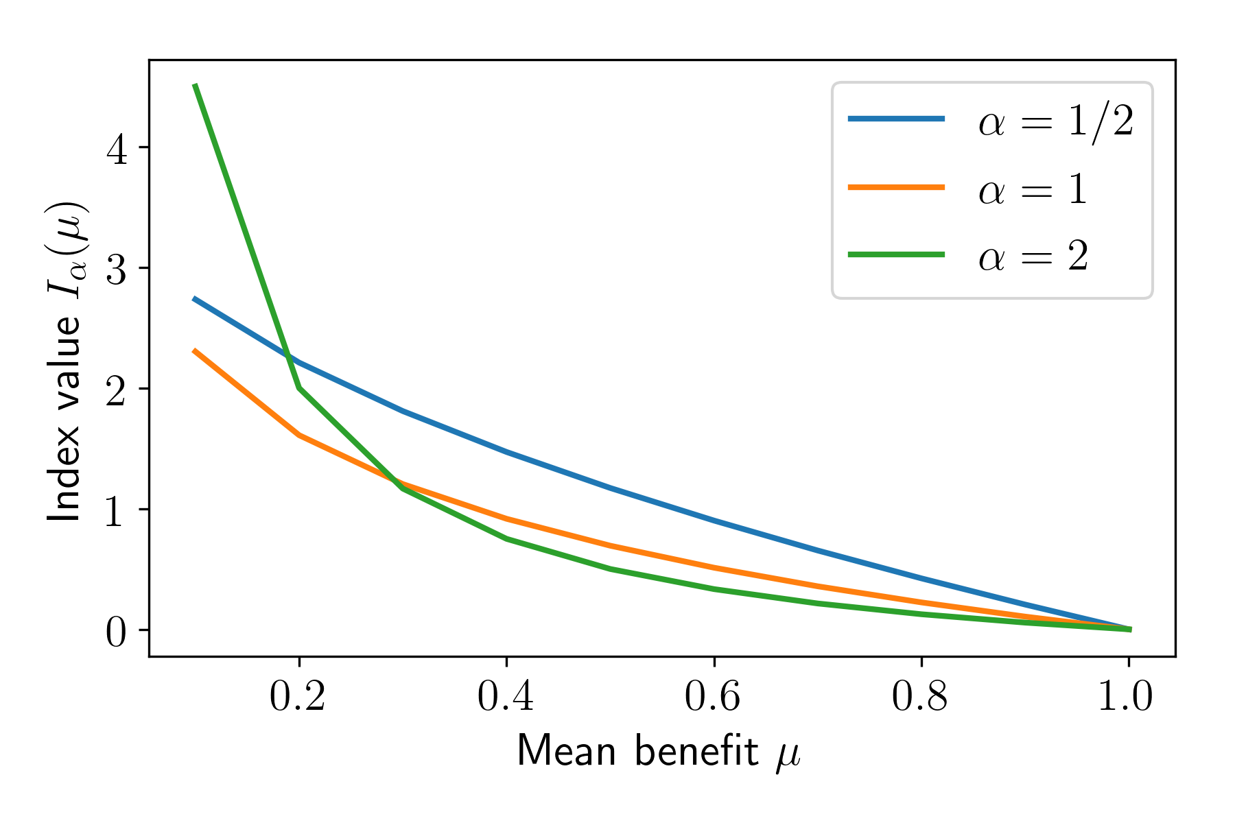
For the benefit functions listed in Table 5.1 the only way to achieve overall fairness (index value zero) is if every individual under consideration receives a benefit of exactly one. We showed this to be the case for binary benefits above. For the fairness criterion in the last row of Table 5.1, comparing luck, benefits are no longer binary. We can also achieve a zero index value if all individuals receive a benefit of two; but this is only possible in the degenerate case where all predictions are false positives, that is, \(\hat{Y}=1\) and \(Y=0\). For each benefit function, the scenarios for which overall fairness is minimal (all individuals under consideration receive exactly one benefit) differs.
Comparing Outcomes
For benefit functions comparing outcomes, the higher the acceptance rate, the lower the value of the index. We achieve a perfectly fair model (zero index value) only by accepting everyone. Recall in the previous chapter where our model was stochastic, we saw that treating every individual the same, corresponded to mapping all individuals to the same the distribution over outcomes. Here, the only way to treat all individuals the same, is to accept them all. Notice that our metric is undefined in the case where we reject all individuals.
Comparing Errors
In the case where we translate group fairness criterion comparing errors, the accurate prediction is always defined as the beneficial one. In all cases we can achieve a zero index value with a 100% accurate model, i.e. \(\hat{Y}=Y\). For the benefit function corresponding to equal accuracy, our index is a monotonic function of accuracy and we can only achieve a zero index value, with a 100% accurate model. Neglecting to consider all the points means that in some cases, achieving 100% accuracy is no longer the only way to minimise the index. For example, consider the benefit function corresponding to equal false positive rates. For this we achieve a zero index value so long as the false positive rate is zero. Similar arguments apply to the benefit function corresponding to equal false negative rate, we need the false negative rate to be zero. We leave it to the reader to consider the remaining benefit functions in the Table 5.1.
Equal Luck
The final row of Table 5.1 shows the benefit function proposed by Speicher, Heidari et al. which distinguishes between false negative and false positive errors. We describe the criterion as requiring equal luck. It assumes a positive outcome to be the most advantageous to the individual. It assigns false negative predictions a benefit of zero (the least lucky), while a false positive prediction (the most lucky) is deemed twice as beneficial as a correct prediction. The benefits in this case are a measure of the discrepancy between the individuals assigned label (prediction) and the label deserved according to the ground truth. In fact the benefit is exactly one plus the error, i.e. \(b_i=\hat{y}_i-y_i+1\). It provides a measure of the relative prevalence of false positive to false negative errors; that is, if the model over or underestimates on average.
In the original paper the index value corresponding to equal luck is described as a measure of individual fairness in that "individuals deserving similar outcomes, receive similar outcomes". Recall that individual fairness (as described by Dwork et. al.[59] and discussed in the previous chapter), is the notion that in a fair system, similar people are treated similarly. For the benefit function associated with equal luck, the similarity of individuals is based solely on their associated error, \(\hat{y}_i-y_i\) (and not on their features, as described by Dwork et. al.[59]). The metric looks at the difference between the prediction and ground truth and thus clearly some measure of model performance. As demonstrated earlier, generalised entropy indices are subgroup decomposable loss functions and thus some measure of utility. That said, generalised entropy indices are a measure of individual fairness on some level, albeit one that makes a coarse comparison of individuals and places absolute faith in the data.
5.3.3 Overall Fairness as Utility
We know that for the benefit function corresponding to equal accuracy the index is a monotonic decreasing function of \(\mu\) accuracy. Here the assumption is that false positives and false negatives are equally undesirable. For example consider the binary gender recognition systems reviewed in the project gender shades. In this case the beneficial outcome is a correct prediction. Erroneous predictions (regardless of one’s gender) are never more beneficial than correct predictions. We also know that for both equal accuracy and equal luck benefit functions, the only way to achieve an index value of zero is to have a perfectly accurate solution. It seems like (at least in these two cases), equalising benefits (minimising the index) corresponds to maximising utility (minimising the expected cost). In this case, different choices of benefit function correspond to different costs associated with different predictions, and different choices of \(\alpha\) correspond to different loss functions.
The desirability of a given classification will, in general, depend on one’s perspective. For example, take an algorithm that predicts credit risk, and thus which interest rate (of two - high or low), a given loan applicant is eligible for. Low risk individuals are offered a low interest rate loan, while high risk customers are offered a high interest rate loan. From the perspective of the applicant, being labelled low risk will always be more desirable than being labelled high risk. From the perspective of the bank however, it would be undesirable to label high risk individuals as low risk. If we are interested in the perspective of the individual and we assume \(\hat{Y}=1\) to be the advantageous outcome, then our benefit function \(\mathrm{benefit}(\hat{y}=i, y=j)=b_{ij}\) must satisfy the following constraints \(b_{10}>b_{00}\) and \(b_{11}>b_{01}\). This is because, from the perspective of the individual, a low interest rate loan (\(\hat{y}=1\)) will always be better than a high interest rate loan (\(\hat{y}=0\)), regardless of the actual risk level the individual presents.
In the case, where \(\hat{Y}=1\) is the more advantageous outcome, the least beneficial prediction should be a false negative prediction, where despite presenting low risk, the individual is assigned to the high risk pool. From the perspective of the individual, nothing could be worse. False negative predictions then, should be assigned the minimum possible benefit, that is, \(b_{01}=0\). Thanks to the property of scale invariance (multiplying all the benefits in our matrix by a constant does not change the value of the index), we can choose any non-zero positive value for \(b_{11}>b_{01}=0\). In fact, all other benefits in the matrix should be greater than zero (to choose \(b_{00}=b_{01}\) would be to ignore the information provided by \(Y\)). We choose \(b_{11}=1\). So, for our 2x2 benefit matrix representing individual fairness, we have two degrees of freedom: \[\mathrm{benefit}(\hat{y}=i,y=j) = b_{ij} = \left( \begin{array}{cc} b_{00} & 0 \\ b_{10} & 1 \end{array} \right)\] where \(b_{10}>b_{00}>0\). The remaining benefits in the matrix \(b_{00}\) and \(b_{10}\) establish how beneficial they are relative a true positive prediction.
Suppose we restrict ourselves to the case where accurate predictions are equally beneficial (neither lucky nor unlucky), that is \(b_{00}=b_{11}=1\). Then in general, the benefit function that maps predictions to luck is characterised with a single parameter (the false positive benefit). \[\mathrm{benefit}(\hat{y}=i,y=j) = b_{ij} = \left( \begin{array}{cc} 1 & 0 \\ b_+ & 1 \end{array} \right)\] Note that the benefit function equal accuracy, corresponds to the special case \(b_+=0\), where all types of errors are equally unlucky. The value of our inequality index is computed much like an expected cost. The associated cost matrix is given by, \[c_{ij} = \mathrm{cost}(\hat{y}=i, y=j) = b_{ij}/\mu.\] The difference here is that the associated cost matrix is not constant, but rather depends on the distribution of benefits. Our choice of parameter \(\alpha\), corresponds to different loss functions. As our model performance changes, so does the mean benefit and thus the associated costs. The mean benefit \(\mu\) is always positive and so does not affect the relative size or ordering of the associated costs in the matrix, but can still impact the relative preference of different predictions (as is the case when we define a cost sensitive utility). Crucially, cost sensitive utilities mean that making a more accurate prediction might not always reduce the expected cost.
5.4 Fairness as Utility
In section 5.2.5 we saw how the value of the generalised entropy index is maximal when only one individual benefits. In this section we will show that the distribution of benefits and thus the index are more tightly constrained for any reasonable model \(\hat{Y}\), and that those constraints become tighter still on fixing the dataset. We derive an analytical account of the behaviour of the index given by the criterion of equal luck for different values of \(\alpha\), and show how it relates to other well known model performance metrics.
Under the criterion of equal luck, our benefit distribution can be characterised with three parameters, the mean benefit \(\mu\) and the model accuracy \(\lambda\), and the false positive benefit \(b_+\).
Index value for Equal Luck
| \[ I_{\alpha}\left(\mu,\lambda\right) = \left\{ \begin{array}{cl} \ln \left(\dfrac{b_+}{\mu}\right) - \dfrac{\lambda}{\mu}\ln b_+ & \textrm{if}\quad\alpha = 1 \\ \rule{0em}{4.5ex} \dfrac{1}{\alpha(\alpha-1)} \left[ \left(\dfrac{b_+}{\mu}\right)^{\alpha-1} - \dfrac{(b_+^{\alpha-1}-1)}{\mu^{\alpha}}\lambda - 1 \right] & \textrm{if}\quad \alpha>0. \end{array}\right.\] | (5.12) |
To make the analysis easier in the case where \(\hat{Y}=1\) is the advantageous outcome, we examine the behaviour for the specific case \(b_+=2\), (as suggested in the original paper and specified in Table 5.1). Here the false positive benefit is twice as lucky as an accurate prediction. The mean benefit \(\mu\) here, gives us an indication of the relative number of false positive to false negative errors, made by the model; it tells us if the model is over or underestimating the target on average. From another point of view, it quantifies the amount of skew in the distribution of luck. Skew describes the extent of asymmetry in a distribution. For negatively skewed distributions, the tail is longer (and thinner) on the left (and vice versa for positively skewed distributions). Therefore, \(\mu<1\) indicates more weight on the left (and thus the tail on the right) hence positive skew (and vice versa for \(\mu>1\)). Figure 5.6 provides visual illustrations of benefit distributions with different mean benefits \(\mu\). When the mean benefit is one (as in the centre figure), the distribution has no skew; it is symmetric.
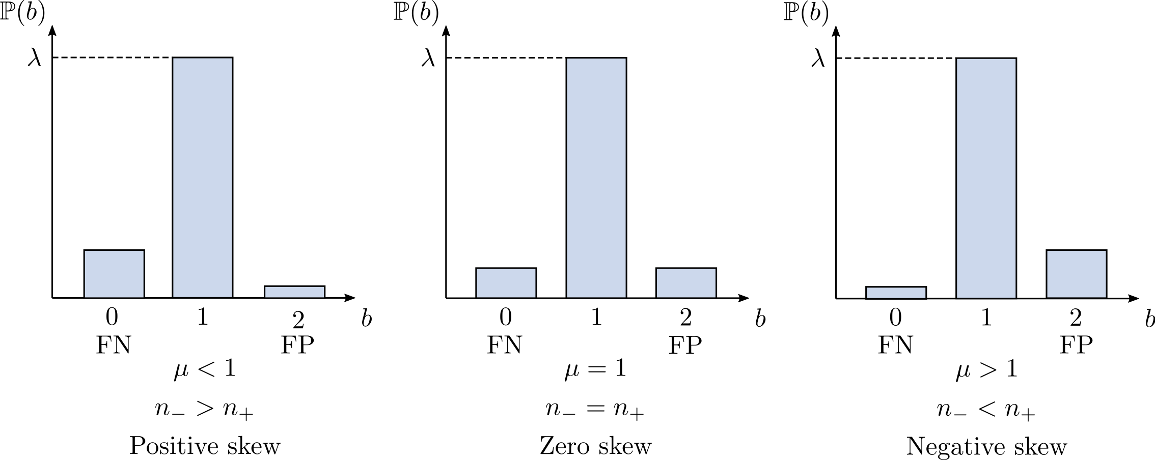
We can see from these equations that for fixed \(\mu\), \(I_{\alpha}(\mu,\lambda)\) is a linearly decreasing function of accuracy. We know that for most problems, the accuracy of our model is bounded below by our dataset, \[0.5 \leq \max[\mathbb{P}(Y=0), \mathbb{P}(Y=1)] < \lambda \leq 1.\] If we can find the maximal value of the index for a given accuracy, this allows us to find an upper bound for the index, based on a dataset with known \(Y\). Before analysing the behaviour of the index as a function of \(\mu\), we note that \(\mu\) is also constrained for our classifier. For a model with accuracy \(\lambda=n_c/n\), the total number of benefits \(B\), must satisfy the following bounds, \[n_c \leq B \leq n_c+2(n-n_c) = 2n-n_c.\] We also know, that the total number of benefits must equate to \(n\) times the mean, that is, \(B=n\mu\). Given this, it is straightforward to show that we must have
| \[ \lambda \leq \mu \leq 2 - \lambda.\] | (5.13) |
As the accuracy of the model \(\lambda\) increases, the range of possible values the mean benefit \(\mu\) can take, decreases. Our domain is then an isosceles triangle. In Figure 5.7 we provide a visualisation of the domain space. We choose to plot the mean benefit \(\mu\) on the horizontal axis, enabling us to visualise the benefit distributions in the natural orientation.
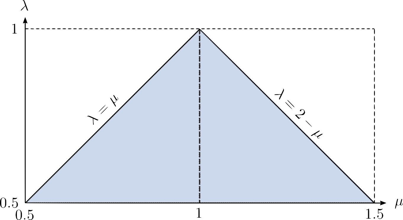
In Figures 5.8 we plot \(I_{\alpha}(\mu,\lambda)\) as a function of \(\mu\) for a range of values of \(\lambda\). Each plot corresponds to a different value of \(\alpha\).
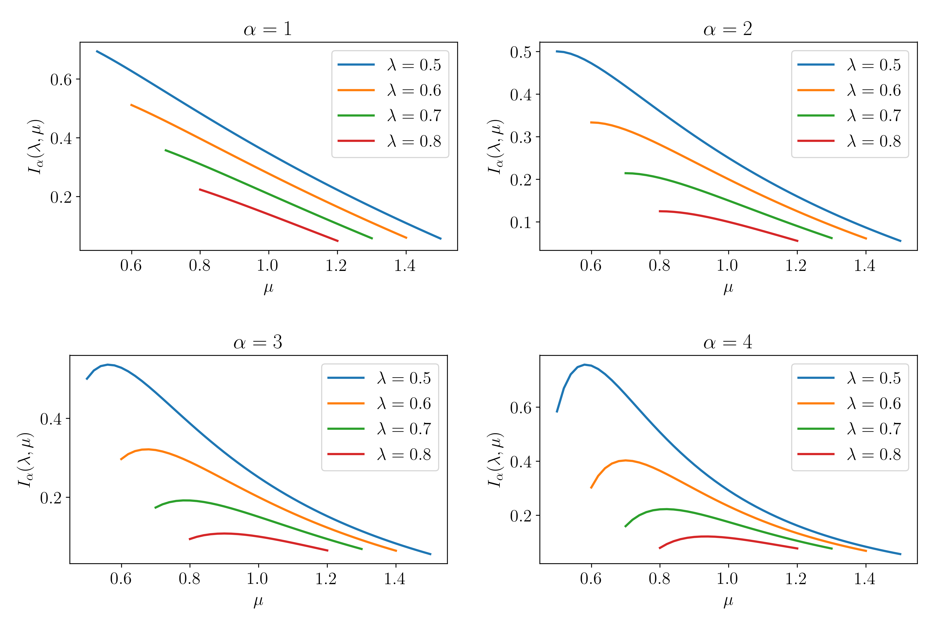
5.4.1 Index maximum
Index turning point
The index has exactly one turning point (a maxima) for \(\alpha>0\), at \(\mu=\tilde{\mu}\) where, \(\tilde{\mu} = g(\alpha)\lambda\) and,
| \[ \quad g(\alpha) = \left\{ \begin{array}{cl} \ln2 & \textrm{if}\quad\alpha = 1 \\ \rule{0em}{3.8ex} \dfrac{\alpha(2^{\alpha-1}-1)}{(\alpha-1)2^{\alpha-1}} & \textrm{if}\quad \alpha>0 \end{array}\right.\] | (5.14) |
Let’s summarise what we know about the behaviour of the index as a function of \(\mu\). \[\begin{aligned} \tilde{\mu}\leq\lambda & \quad\Rightarrow\quad I_{\alpha}(\mu,\lambda) \textrm{ is a strictly decreasing function of }\mu.\\ \lambda<\tilde{\mu}<2-\lambda & \quad\Rightarrow\quad I_{\alpha}(\mu,\lambda) \textrm{ is maximal at }\mu=\tilde{\mu}=g(\alpha)\lambda.\\ \tilde{\mu}\geq2-\lambda & \quad\Rightarrow\quad I_{\alpha}(\mu,\lambda) \textrm{ is a strictly increasing function of }\mu. \end{aligned}\]
From equations (5.13) and (5.14), we see that for \(\tilde{\mu}\) to fall within the domain of \(\mu\) we require,
| \[ \lambda \leq g(\alpha)\lambda \leq 2 - \lambda \quad\Leftrightarrow\quad 1 < g(\alpha) < \frac{2}{\lambda}-1.\] | (5.15) |
For convenience, we reformulate the upper bound on \(g(\alpha)\) as a bound on \(\lambda\).
| \[ g(\alpha) < \frac{2}{\lambda}-1 \quad\Leftrightarrow\quad \lambda < \tilde{\lambda}(\alpha) = \frac{2}{1+g(\alpha)},\] | (5.16) |
where \(g(\alpha)\) is given in equation 5.14. To understand the behaviour of the index better, we need to understand the behaviour of \(g(\alpha)\) and \(\tilde{\lambda}(\alpha)\). We plot \(g(\alpha)\) and \(\tilde{\lambda}(\alpha)\) in Figures 5.9.
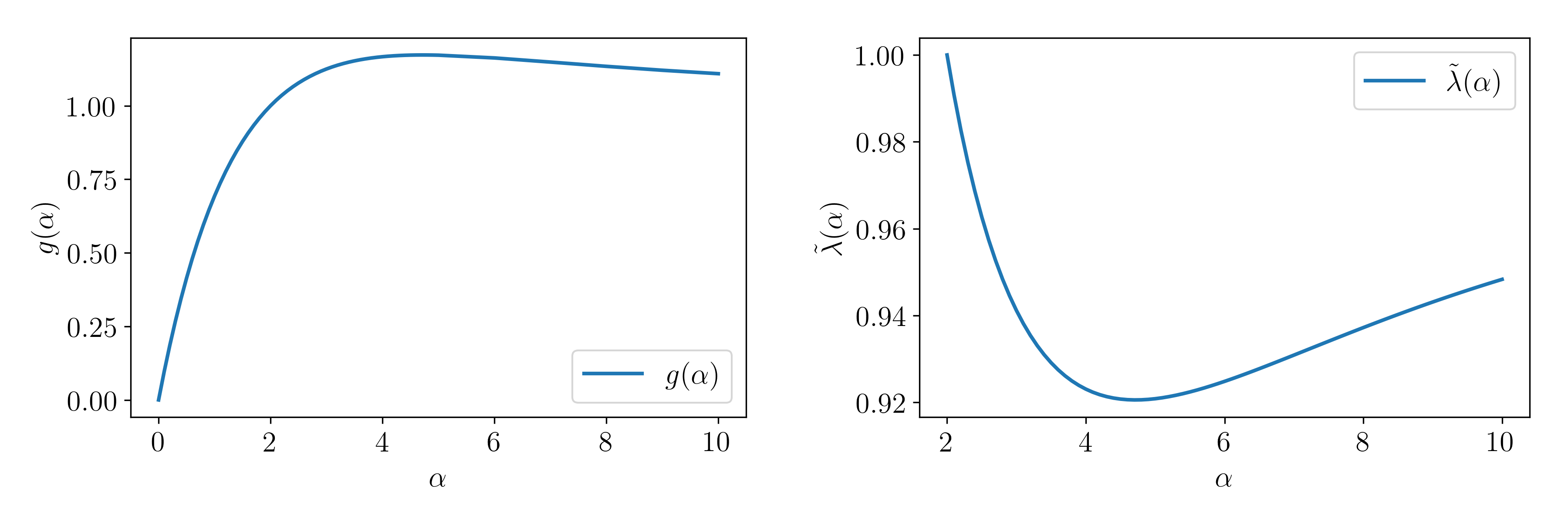
Note that, \[g(2)=1 \quad\textrm{and}\quad\left\{ \begin{array}{lcr} g(\alpha)<1 & \textrm{if} & 0<\alpha<2,\\ g(\alpha)>1 & \textrm{if} & \alpha>2. \end{array}\right.\] This allows us to reformulate the lower bound on \(g(\alpha)\) (given in equation (5.15)) as bound on \(\alpha\), \[g(\alpha) > 1 \quad\Leftrightarrow\quad \alpha > 2.\] Since \(2^{\alpha-1}\) dominates \(\alpha\) for large \(\alpha\), we know that \[g(\alpha) \rightarrow 1^+ \quad\textrm{as}\quad \alpha\rightarrow\infty \quad\Rightarrow\quad\tilde{\lambda}(\alpha) \rightarrow 1^- \quad\textrm{as}\quad \alpha\rightarrow\infty.\] Differentiating \(g(\alpha)\) in equation (5.14) gives, \[g'(\alpha) = \frac{\alpha(\alpha-1)\ln2 - (2^{\alpha-1}-1)} {[(\alpha-1)2^{\alpha-1}]^2}=0 \quad\Leftrightarrow\quad \alpha = \alpha_*\] where \(\alpha_*\) satisfies \[\alpha_*(\alpha_*-1)\ln2 = 2^{\alpha_*-1}-1.\] \(g'(\alpha)\) has exactly one root \(\alpha=\alpha_*\) (somewhere between 4 and 5) which can be found numerically. \[g''(\alpha_*) = \frac{2-\alpha_*\ln2}{(\alpha_*-1)2^{\alpha_*-1}} < 0.\] Thus \(g(\alpha)\) is maximal at \(\alpha=\alpha_*\). For reference, \[\begin{aligned} \alpha_* \approx 4.72 \quad\Rightarrow\quad & \max_{\alpha>0}[g(\alpha)] = g(\alpha_*) \approx 1.17 \\ \Rightarrow\quad & \min_{\alpha>0}[\tilde{\lambda}(\alpha)] = \tilde{\lambda}(\alpha_*) \approx 92.1\%. \end{aligned}\] We can now summarise the behaviour of the index for a given model accuracy, in terms of our metric inputs (\(\lambda\) and \(\alpha\)). \[\begin{aligned} \alpha\leq2 \phantom{\textrm{ and }\lambda<\tilde{\lambda}} & \quad\Rightarrow\quad I_{\alpha}(\mu,\lambda) \textrm{ is a strictly decreasing function of }\mu, \textrm{ maximal at }\mu=\lambda.\\ \alpha>2\textrm{ and }\lambda<\tilde{\lambda} & \quad\Rightarrow\quad I_{\alpha}(\mu,\lambda) \textrm{ is maximal at }\mu=g(\alpha)\lambda.\\ \alpha>2\textrm{ and }\lambda\geq\tilde{\lambda} & \quad\Rightarrow\quad I_{\alpha}(\mu,\lambda) \textrm{ is a strictly increasing function of }\mu, \textrm{ maximal at }\mu=2-\lambda. \end{aligned}\] where \(g(\alpha)\) and \(\tilde{\lambda}\) are given in equations (5.14) and (5.16) respectively. These characteristically different behaviours are indeed observed in Figures 5.8 for different values of \(\alpha\) and \(\lambda\). We note that in these plots, the accuracy \(\lambda\) does exceed the level required, for the index to become a strictly increasing function of \(\mu\). For reference, \(\tilde{\lambda}(3)=16/17\approx94.1\%\) and \(\tilde{\lambda}(4)=12/13\approx92.3\%\).
We are almost there. We now know that, \[\max_{\mu}\left[I_{\alpha}\left(\mu,\lambda\right)\right] = I_{\alpha}\left(\mu_*,\lambda\right) \nonumber\\ \] where, \[\mu_* = \left\{ \begin{array}{cl} \lambda & \quad\textrm{if}\quad 0<\alpha\leq2 \\ g(\alpha)\lambda & \quad\textrm{if}\quad \alpha>2 \quad\textrm{and}\quad \lambda<\tilde{\lambda}(\alpha) \\ 2-\lambda & \quad\textrm{if}\quad \alpha>2 \quad\textrm{and}\quad \lambda\geq\tilde{\lambda}(\alpha). \end{array}\right.\] Substituting \(\mu=\mu_*\) into equation (5.12) yields the index maximum (for fixed \(\alpha\) and \(\lambda\)),
Equal Luck Generalised Entropy Index Maximum Value
We can write the maximal value of the generalised entropy index as a function of \(\lambda\), \[\max_{\mu}\left[I_{\alpha}\left(\mu,\lambda\right)\right] = \left\{ \begin{array}{cl} -\ln\lambda & \textrm{if}\quad \alpha=1 \\ \rule{0em}{4.1ex} \dfrac{1}{\alpha(\alpha-1)}\left(\dfrac{1}{\lambda^{\alpha-1}} - 1 \right) & \textrm{if}\quad 0<\alpha\leq2 \\ \rule{0em}{4.1ex} \dfrac{1}{\alpha(\alpha-1)}\left[\dfrac{2^{\alpha-1}} {\alpha g^{\alpha-1}(\alpha)\lambda^{\alpha-1}} - 1 \right] & \textrm{if}\quad \alpha>2,\,\lambda<\tilde{\lambda}(\alpha) \\ \rule{0em}{4.1ex} \dfrac{1}{\alpha(\alpha-1)} \left(\dfrac{1}{(2-\lambda)^{\alpha-1}} - 1 \right) & \textrm{if}\quad \alpha>2,\,\lambda\geq\tilde{\lambda}(\alpha) \end{array}\right.\] where, \[\tilde{\lambda}(\alpha) = \frac{2}{1+g(\alpha)} \quad\textrm{and}\quad g(\alpha) = \left\{ \begin{array}{cl} \ln2 & \textrm{if}\quad\alpha = 1 \\ \rule{0em}{3.8ex} \dfrac{\alpha(2^{\alpha-1}-1)}{(\alpha-1)2^{\alpha-1}} & \textrm{if}\quad \alpha>0 \end{array}\right.\]
In Figures 5.10 we plot \(I_{\alpha}(\mu,\lambda)\) as a function of \(\mu\) for a range of values of \(\alpha\). Each plot corresponds to a different value of \(\lambda\). In the final plot, \(\lambda=95\%\); we see that \(I_{\alpha}(\mu,\lambda)\) is a strictly increasing function of \(\mu\), for both \(\alpha=3\) and \(\alpha=4\).
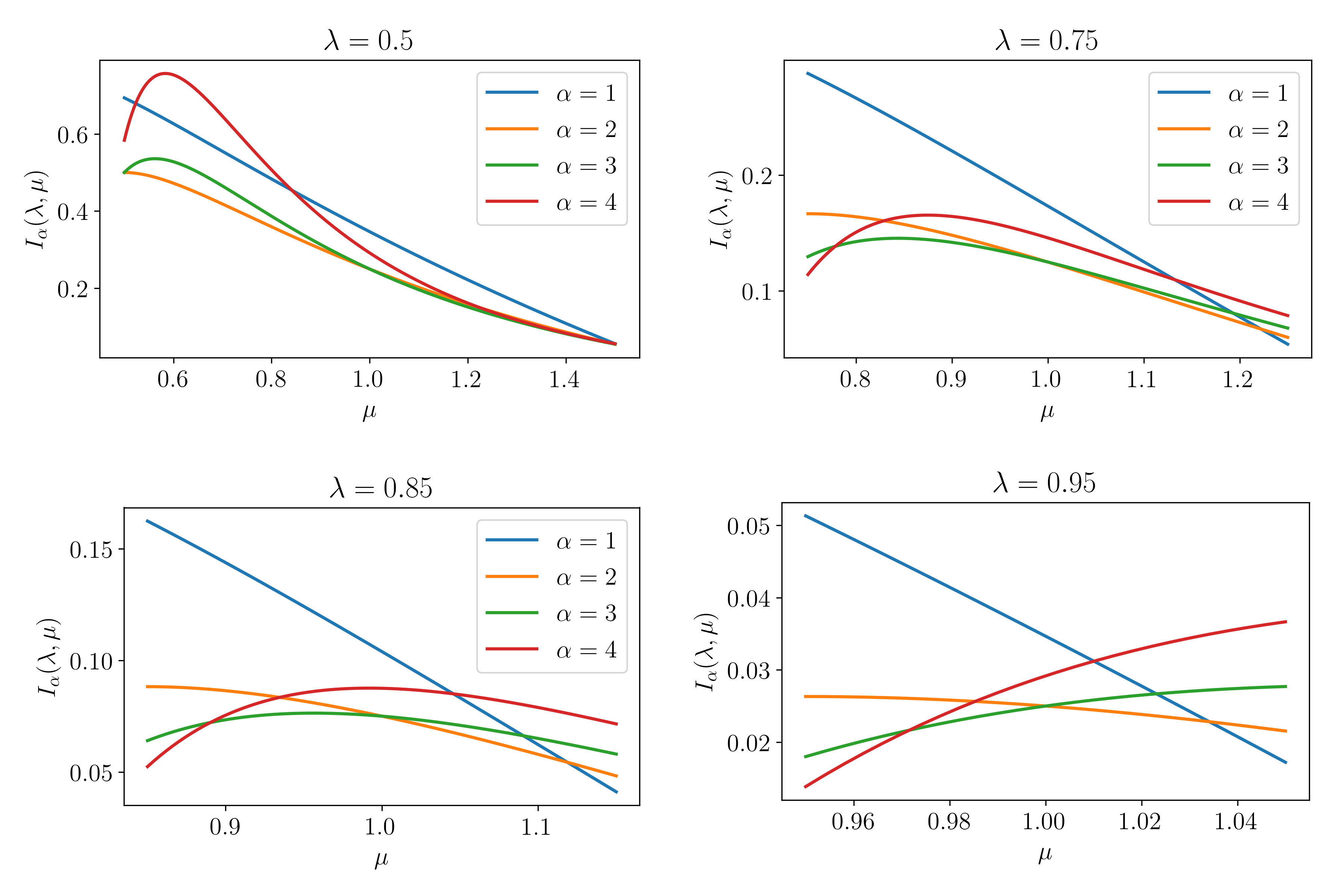
From Figure 5.10, we can see that both \(\lambda\) and \(\alpha\), have an impact on the relative preference between false positive and false negative errors. As the accuracy of our model increases, the change in behaviour of the index, for different choices of \(\alpha\), becomes more extreme.
5.4.2 When is Making an Error Preferable?
The final task in our analysis if the inequality index implied by equal luck, is to calculate the cost of an error. In particular, we want to know when increasing the accuracy of a model does not correspond to reducing the value of the index. For a binary classifier, the space of possible benefit distributions is constrained. We cannot arbitrarily transfer benefits from rich to poor. The range of possible benefits an individual \(i\) can receive is limited by their value \(y_i\). If \(y_i=0\) then \(b\in\{1,2\}\), but if \(y_i=1\) then \(b\in\{0,1\}\).
The Cost of an Error
Let us denote the cost of an error as, \[\Delta I^{\pm}_{\alpha}(\boldsymbol{b}) = I_{\alpha}(\boldsymbol{b^{\pm}}) - I_{\alpha}(\boldsymbol{b}).\] Here \(\boldsymbol{b^{\pm}}\) differs from \(\boldsymbol{b}\) by one prediction only, containing one less correct prediction, and one more erroneous one. For \(\boldsymbol{b^{+}}\), the additional error is a false positive. For \(\boldsymbol{b^{-}}\), the additional error is a false negative. An additional false negative error, reduces the total benefits by one; both the accuracy \(\lambda\) and the mean benefit \(\mu\) are reduced by \(1/n\). An additional false positive error, increases the total benefits by one; the accuracy \(\lambda\) is, once again, reduced by \(1/n\), and the mean benefit \(\mu\) increases by \(1/n\). Therefore, we can write,
| \[ \Delta I^{\pm}_{\alpha}(\mu,\lambda;n) = I_{\alpha}\left(\lambda-\frac{1}{n}, \mu\pm\frac{1}{n}\right) - I_{\alpha}(\mu,\lambda).\] | (5.17) |
The discrete grid of adjacent models we can reach through a small change in the model (given \(\mu\), \(\lambda\) and \(n\)), is shown in Figure 5.11.
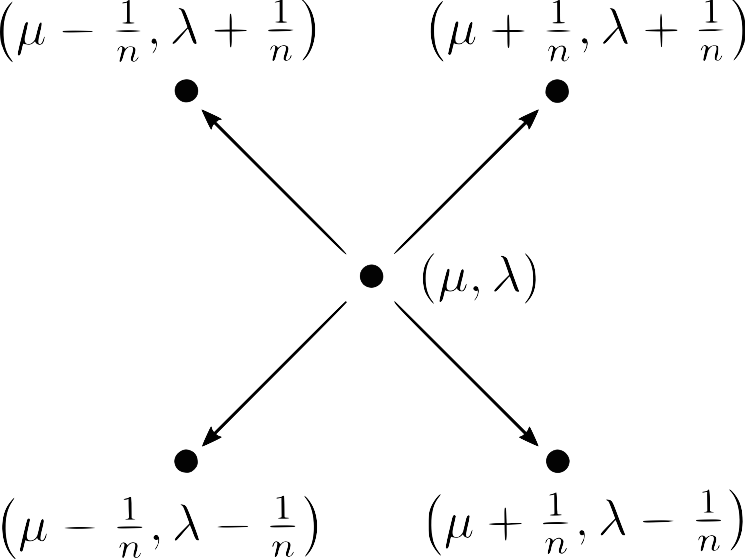
Equation 5.12 provides an expression for \(I_{\alpha}(\mu,\lambda)\). Substituting for \(\lambda\) and \(\mu\) in the case \(\alpha=1\) gives, \[I_{\alpha}\left(\lambda-\frac{1}{n},\mu\pm\frac{1}{n}\right) = \left[1-\left(\frac{\lambda}{\mu}-\frac{1}{n\mu}\right) \left(1\pm\frac{1}{n\mu}\right)^{-1}\right]\ln2-\ln\mu - \ln\left(1\pm\frac{1}{n\mu}\right).\] For \(\alpha>0\), we get, \[I_{\alpha}\left(\lambda-\frac{1}{n},\mu\pm\frac{1}{n}\right) = \frac{1}{\alpha(\alpha-1)} \left[ \left(\frac{2}{\mu}\right)^{\alpha-1} \left(1\pm\frac{1}{n\mu}\right)^{1-\alpha} - \frac{(2^{\alpha-1}-1)}{\mu^{\alpha-1}} \left(\frac{\lambda}{\mu}-\frac{1}{n\mu}\right) \left(1\pm\frac{1}{n\mu}\right)^{-\alpha} - 1 \right].\] We showed earlier that we must have, \(\lambda\leq\mu\leq2-\lambda\), in addition, for most problems, any reasonable model should have \(0.5\leq\lambda\leq1\). We deduce that we must have \(0.5\leq\mu\leq1.5\) and so \(\mu=\mathrm{O}(1)\). Then for large \(n\), we can be sure that \(n\mu\) is large and its reciprocal is small. For large \(n\), we can write the cost of an error as \[\Delta I^{\pm}_{\alpha}(\mu,\lambda;n) = \xi_{\alpha}(\mu,\lambda) \left(\frac{1}{n\mu}\right) + \mathrm{O}\left(\frac{1}{n\mu}\right)^2\] where, \[\xi_{\alpha}(\mu,\lambda) = \left\{ \begin{array}{cl} \left(1\pm\dfrac{\lambda}{\mu}\right)\ln2\mp1 & \textrm{if}\quad\alpha = 1 \\ \rule{0em}{4.1ex} \dfrac{1}{\alpha(\alpha-1)\mu^{\alpha}}\bigg[ \Big((1\pm1\mp\alpha)2^{\alpha-1}-1\Big)\mu \pm \alpha(2^{\alpha-1}-1)\lambda\bigg] & \textrm{if}\quad \alpha>0. \end{array}\right.\]
From these expressions, we can get a clearer understanding of when the index deviates from simply being a measure of error. In particular, we want to know when an error, is preferable to an accurate prediction; that is, when the index change (resulting from an error) is negative. With a little effort we can show that,
| \[ \left. \begin{array}{cl} & \Delta I^-_{\alpha}(\mu,\lambda;n) < 0 \quad\Rightarrow\quad \mu < h^-(\alpha) \lambda \\ & \Delta I^+_{\alpha}(\mu,\lambda;n) < 0 \quad\Rightarrow\quad \mu > h^+(\alpha) \lambda \end{array}\qquad\right\}\] | (5.18) |
where,
| \[ h^{\pm}(\alpha) = \left\{ \begin{array}{cl} \dfrac{\ln2}{1\mp\ln2} & \textrm{if}\quad\alpha = 1 \\ \rule{0em}{4.1ex} \dfrac{\alpha(2^{\alpha-1}-1)}{(\alpha-1\mp1)2^{\alpha-1}\pm1} & \textrm{if}\quad \alpha>0 \end{array}\right.\] | (5.19) |
False Negative Errors
Let’s start by looking at \(h^-(\alpha)\), which we re-write as,
| \[ h^-(\alpha) = \left\{ \begin{array}{cl} \dfrac{\ln2}{1+\ln2} \approx 0.41 & \textrm{if}\quad\alpha = 1 \\ \rule{0em}{4.1ex} 1-\dfrac{\alpha-1}{\alpha2^{\alpha-1}-1} & \textrm{if}\quad \alpha>0 \end{array}\right.\] | (5.20) |
Equation (5.20) reveals that \(h^-(\alpha)\) is a strictly increasing function of \(\alpha\), for \(\alpha>0\) (since \(\alpha2^{\alpha-1}\) dominates \(\alpha\)). In addition, we can see that \(h^-(\alpha)\rightarrow1^-\) as \(\alpha\rightarrow\infty\). In Figure 5.12 we plot \(h^-(\alpha)\).
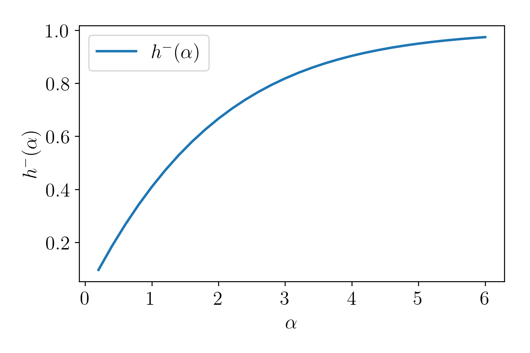
Earlier we showed that we must have \(\mu\geq\lambda\). Then from equation (5.18), for \(\Delta I^-_{\alpha}(\mu,\lambda;n)<0\) we need \(h^-(\alpha)>1\). Since \(h^-(\alpha)<1\) for all \(\alpha>0\), we know that making an additional false negative error, never decreases the value of the index. What about false positive errors?
False Positive Errors
We rewrite \(h^+(\alpha)\) as,
| \[ h^+(\alpha) = \left\{ \begin{array}{cl} \dfrac{\ln2}{1-\ln2} \approx 2.26 & \textrm{if}\quad\alpha = 1 \\ \rule{0em}{4.2ex} \dfrac{\alpha(1-2^{1-\alpha})}{(\alpha-2)+2^{1-\alpha}} & \textrm{if}\quad \alpha>0. \end{array}\right.\] | (5.21) |
Equation (5.21) reveals that \(h^+(\alpha)\) is a decreasing function of \(\alpha\), since \(2^{1-\alpha}\) is a strictly decreasing function of \(\alpha\). In addition, we can see that \(h^+(\alpha)\rightarrow1^+\) as \(\alpha\rightarrow\infty.\) Earlier we showed that we must have \(\mu\leq2-\lambda\). Then from equation (5.18), for \(\Delta I^+_{\alpha}(\mu,\lambda;n)<0\) we need, \[h^+(\alpha)\lambda < 2-\lambda \quad\Leftrightarrow\quad \lambda < \bar{\lambda}(\alpha) = \frac{2}{1+h^+(\alpha)}.\] From what ew know about \(h^+(\alpha)\), we can deduce that \(\bar{\lambda}(\alpha)\) is an increasing function of \(\alpha\), and \(\bar{\lambda}(\alpha)\rightarrow1^-\) as \(\alpha\rightarrow\infty\). Since \(\bar{\lambda}(\alpha)<1\) for all \(\alpha>0\), we know there are indeed some circumstances, under which a false positive error, decreases the value of the index. In Figures 5.13, we plot \(h^+(\alpha)\) and \(\bar{\lambda}(\alpha)\).
![Figure 5.13: h^+(\alpha)=[\alpha(2^{\alpha-1}-1)]/[(\alpha-2)2^{\alpha-1}+1]\quad and \quad\bar{\lambda}(\alpha)=2/[1+h^+(\alpha)].](05_UtilityFairness/figures/Fig_h_plus_lambda_bar_alpha.png)
The Deviation Region
We call the deviation region the part of the domain for which the index is not reduced by reducing the error rate, but instead reduced by increasing the error rate. For our benefit function equal luck, \[I_{\alpha}(\mu,\lambda): ([\lambda, 2-\lambda], [0.5,1]) \mapsto \mathbb{R}_{\geq0}.\] The only kind of error which is ever preferable to a correct prediction under this benefit function is a false positive error. This happens only when the mean benefit exceeds \(h^+(\alpha)\lambda\), that is when the ratio of lucky to unlucky people is sufficiently high. We note that for a model whose accuracy is greater than \(\bar{\lambda}(\alpha)\), it is not possible for the mean benefit (skew) to exceed the required level. That is, \[\begin{aligned} & \Delta I^-_{\alpha}(\mu,\lambda;n) > 0 \quad \forall\,\mu, \,\lambda, \, n \\ & \Delta I^+_{\alpha}(\mu,\lambda;n) < 0 \quad\Rightarrow\quad \mu > h^+(\alpha) \lambda \end{aligned}\] where, \[h^+(\alpha) = \left\{ \begin{array}{cl} \dfrac{\ln2}{1-\ln2} \approx 2.26 & \textrm{if}\quad\alpha = 1 \\ \rule{0em}{4.2ex} \dfrac{\alpha(2^{\alpha-1}-1)}{(\alpha-2)2^{\alpha-1}+1} & \textrm{if}\quad \alpha>0 \end{array}\right.\] This is only possible if the accuracy is sufficiently low, \[\lambda < \bar{\lambda}(\alpha)=\frac{2}{1+h^+(\alpha)}.\] The deviation region is then described as, \(\mu>h^+(\alpha)\lambda\), where \(h^+(\alpha)\) is given in equation (5.21). We mark the deviation region on the contour plot for \(I_{\alpha}(\mu, \lambda)\) in Figure 5.14.
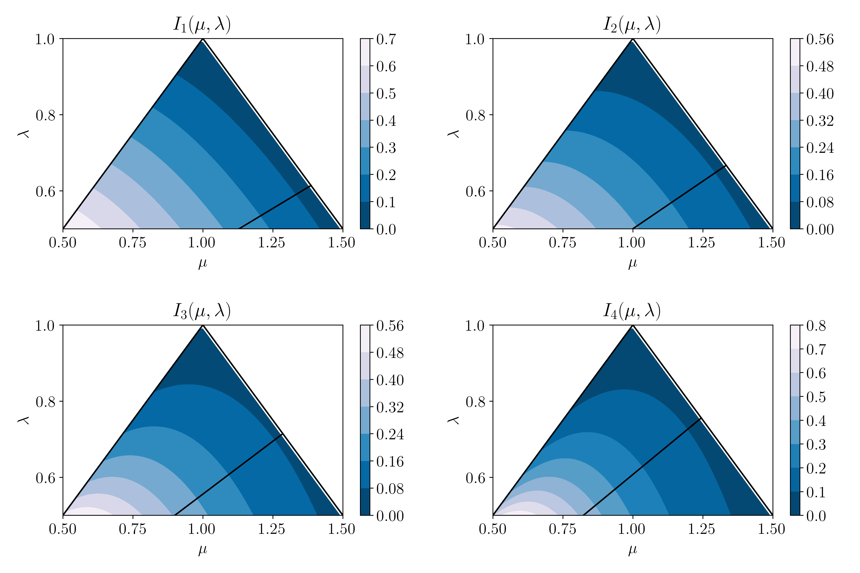
For reference, in Table 5.2, we provide some values of \(\bar{\lambda}(\alpha)\) and \(h^+(\alpha)\).
| \(\alpha\) | \(\bar{\lambda}(\alpha)\)a | \(h^+(\alpha)\)b |
|---|---|---|
| 1 | 61.4% | 2.26 |
| 2 | 66.7% | 2 |
| 3 | 71.4% | 1.8 |
| 4 | 75.6% | 1.65 |
aWe require \(\lambda<\bar{\lambda}(\alpha)\) for the possibility that reducing the index value may not correspond to reducing the error rate. At \(\lambda=\bar{\lambda}(\alpha)\), all the errors must be false positives to achieve the value of \(\mu\) required for \(\Delta I^+(\mu,\lambda;\alpha,n)<0\).
bWe require \(\mu>h^+(\alpha)\lambda\) for a false positive error to result in a reduction of the index value.
Summary
Inequality indices measure divergence from the uniform distribution. We can think of them as a system for ranking distributions from most fair to least fair, the most fair having an index value of zero and becoming more unfair as the value of the index increases.
Note that two distributions that diverge equally from the uniform distribution, need not be the same distribution. Different inequality indices break ties in different ways.
Generalised Entropy Indices
Generalised entropy indices, are a special family of inequality indices that are subgroup decomposable. That is, they can be disaggregated across subgroups of a population, into the sum of a between-group component and a within-group component.
The between-group component is computed as the value of the index, assuming all individuals receive the mean benefit of the partition to which they belong. Essentially, it measures the contribution to the inequality index, from variation in the average benefit between the subgroups (akin to the notion of group fairness we discussed in chapter 3, except here, the relative sizes of the subgroups matter). If all the groups have the same mean benefit the between-group component is zero.
The within-group component is computed as a weighted sum of the index value for each subgroup, and can be thought of as measuring the contribution to overall (individual) unfairness, arising from variation in benefits between individuals in the subgroups. For a within-group component to be zero, we require every individual in the subgroup to have exactly the same benefit.
The ability to additively decompose this inequality measure into intergroup and intragroup components, allows us to identify when trade-offs between the different notions of fairness (between-group and within-group) might occur.
We posit generalised entropy indices as a special family of subgroup decomposable loss functions with generalisation parameter \(\alpha\).
\(\alpha\) controls the weight applied to different parts of the distribution when calculating the loss.
For \(\alpha=0\), the index \(I_0\) is a linear function of the cross entropy loss.
In the special case \(\alpha=1/2\), the contribution to the total loss from the between-group component is maximal.
Defining a Benefit Function
Benefit functions map predictions to benefits \(\mathrm{benefit}(\hat{y}=i,y=j)=b_{ij}\).
In the special case where a accurate predictions are equally beneficial and a false negative yields no benefit, the benefit function might be thought of as a measure of luck (where a false negative error is as unlucky as it gets). In this case luck is characterised with a single parameter (the false positive benefit) \(b_+\geq0\) which tells us how lucky it is relative to an accurate prediction. \[\mathrm{benefit}(\hat{y}=i,y=j) = b_{ij} = \left( \begin{array}{cc} 1 & 0 \\ b_+ & 1 \end{array} \right)\]
The index is computed much like an expected loss on the cost where the cost matrix is given by, \[c_{ij} = \mathrm{cost}(\hat{y}=i, y=j) = b_{ij}/\mu.\]
The cost matrix is not constant, but rather depends on the mean benefit.
Fairness as Utility
For the choice \(b_+=0\),
Only an accurate prediction is lucky; errors correspond to zero luck.
The index is a monotonic decreasing function of the mean benefit (or equivalently model accuracy) \(\mu\), essentially a cost insensitive measure of utility.
For the choice \(b_+=2\),
a false positive is twice as lucky as an accurate prediction. The benefit can be computed as one plus the error, \(b_i=\hat{y}_i-y_i\).
The index can be written as a function of the mean benefit \(\mu\) and model accuracy \(\lambda\). The mean benefit gives an indication of the skew in the distribution of errors. For fixed mean benefit \(\mu\), the index is a linearly decreasing function of the accuracy \(\lambda\).
For any reasonable model and \(\alpha>0\), the value of the index is bounded.
We find that false negative predictions are never more fair than an accurate prediction.
False positive predictions are fairer than accurate predictions when the distribution is sufficiently skewed.
Once the accuracy of a model is sufficiently high, it becomes impossible for the distribution of errors to be sufficiently skewed and the index always decreases with increasing accuracy.
The threshold on skew \(\mu\) for which a false positive is deemed fairer than an accurate prediction, is a decreasing function of \(\alpha\).
A Notation and Conventions
| Letter case &/ Typeface | Denotes |
|---|---|
| Lowercase | Scalar variables, e.g. \(a\) |
| Uppercase | Random variables, e.g. \(X\) |
| Lowercase bold | Vectors, e.g. \(\boldsymbol{y}\) |
| Uppercase bold | Matrices and vectors of random variables e.g. \(\boldsymbol{X}\) |
| Type | Expression | Denotes |
|---|---|---|
| Symbols | \(\forall\) | For all |
| \(|\) | Such that | |
| \(\in\) | Is a member of | |
| \(\Rightarrow\) | Implies | |
| \(\Leftrightarrow\) | If and only if | |
| \(\rightarrow\) | Tends to | |
| \(x\rightarrow a^{\pm}\) | \(x\) tends to \(a\) from above (+) or below (-) | |
| Brackets | \(x \in [a,b)\) | \(a\leq x<b\) (inclusive and exclusive parenthesis) |
| Sets | \(\cup\) | Union, logical OR |
| \(\cap\) | Intersection, logical AND |
| Function | Definition |
|---|---|
| Heaviside step function | \(\displaystyle \phantom{\delta(x)'=} H(x) = \left\{ \begin{array}{rl} 1 & \textrm{if} \quad x > 0 \\ 0 & \textrm{otherwise} \end{array} \right.\) |
| Delta function | \(\displaystyle \delta(x) = H'(x) = \left\{ \begin{array}{cl} \infty & \textrm{if} \quad x=0 \\ 0 & \textrm{otherwise} \end{array} \right.\) |
| Type | Expression | Denotes |
|---|---|---|
| Data size | \(n\) | Number of data points / individuals |
| \(m\) | Number of features (predictive model input size) | |
| Random variables | \(\boldsymbol{X}\) \(\in\mathcal{X}\) | Features: \(\boldsymbol{X}\) \(=(X_1,...,X_m)\) |
| \(\boldsymbol{Z}\) \(\in\mathcal{Z}\) | Sensitive features: gender, race, etc. | |
| \(Y\in\mathcal{Y}\) | Target | |
| \(\hat{Y}=f(\boldsymbol{X})\) | Model predictions \(\hat{y}\) are a function \(f\) of the features \(\boldsymbol{x}\) | |
| Data | \(\boldsymbol{X}\), \(\boldsymbol{Z}\), \(\boldsymbol{y}\) | Data for all \(n\) individuals |
| \(\boldsymbol{x}_i\), \(\boldsymbol{z}_i\), \(y_i\) | Data for individual \(i\). | |
| \(x_{ij}\), \(z_{ij}\) | The element of matrix \(\boldsymbol{X}\) at row and column indices \(i, j\) | |
| \(p(\boldsymbol{x})\) | Regression | |
| \(H(p(\boldsymbol{x})-\tau)\) | Deterministic binary classification | |
| Special values | \(Y = y_{\pm}\) | Advantageous (+) or disadvantageous (-) outcome |
| \(Z = z_{\pm}\) | Privileged / advantaged (+) or disadvantaged (-) class | |
| Metrics | \(d\) | Difference |
| \(r\) | Rate / ratio | |
| Probability | \(\mathbb{P}(A)\) | Probability of event \(A\) |
| \(f_X(x)\) | Probability density function for the random variable \(X\) | |
| Discrete \(X\) | \(\displaystyle \mathbb{P}(x)=\mathbb{P}(X=x)=f_{X}(x)\)a | |
| Continuous \(X\) | \(\displaystyle \mathbb{P}(a\leq X<b)=\int_a^b f_X(x) \, \mathrm{d}x\) | |
| Expectation | \(\mathbb{E}[X)\) | Expected value of random variable \(X\) |
| \(\mathbb{E}[g(X)]\) | \(\displaystyle \sum_{x\in\mathcal{X}} g(x)f_X(x) = \int_{x\in\mathcal{X}} g(x)f_X(x) \, \mathrm{d}x\) | |
| \(\mathbb{E}_X[g(X,Y)]\) | \(\displaystyle \sum_{x\in\mathcal{X}} g(x,y)f_X(x) = \int_{x\in\mathcal{X}} g(x,y)f_X(x) \, \mathrm{d}x\) |
aFor readability, when it is clear from the context, we shall omit the random variable in the event descriptor, for example, \(\mathbb{P}(X=x)=\mathbb{P}(x)\).
B Performance Metrics
Confusion Matrix Metrics
Performance Metrics
| Ground Truth | ||||
|---|---|---|---|---|
| \(y=1\) | \(y=0\) | Metric | ||
| Prediction | \(\hat{y}=1\) | True Positive | False Positive Type I Error |
Positive Predictive Valuea \(\mathbb{P}(\hat{y}=y|\hat{y}=1)\) |
| \(\hat{y}=0\) | False Negative Type II Error |
True Negative | Negative Predictive Value \(\mathbb{P}(\hat{y}=y|\hat{y}=0)\) |
|
| Metric | True Positive Rateb \(\mathbb{P}(\hat{y}=y|y=1)\) |
True Negative Rate \(\mathbb{P}(\hat{y}=y|y=0)\) |
Accuracy \(\mathbb{P}(\hat{y}=y)\) |
|
a Positive Predictive Value = Precision
b True Positive Rate = Recall
Error Metrics
| Ground Truth | ||||
|---|---|---|---|---|
| \(y=1\) | \(y=0\) | Error Rate Type | ||
| Prediction | \(\hat{y}=1\) | True Positive | False Positive Type I Error |
False Discovery Rate \(\mathbb{P}(\hat{y}\neq y|\hat{y}=1)\) |
| \(\hat{y}=0\) | False Negative Type II Error |
True Negative | False Omission Rate \(\mathbb{P}(\hat{y}\neq y|\hat{y}=0)\) |
|
| Error Rate Type | False Negative Rate \(\mathbb{P}(\hat{y}\neq y|y=1)\) |
False Positive Rate \(\mathbb{P}(\hat{y}\neq y|y=0)\) |
Error Rate \(\mathbb{P}(\hat{y}\neq y)\) |
|
Combined table
| Ground Truth | ||||
|---|---|---|---|---|
| Prediction | \(y=1\) | \(y=0\) | Performance | Error rate |
| \(\hat{y}=1\) | True Positive | False Positive Type I Error |
Positive Predictive Valuea \(\mathbb{P}(\hat{y}=y|\hat{y}=1)\) |
False Discovery Rate \(\mathbb{P}(\hat{y}\neq y|\hat{y}=1)\) |
| \(\hat{y}=0\) | False Negative Type II Error |
True Negative | Negative Predictive Value \(\mathbb{P}(\hat{y}=y|\hat{y}=0)\) |
False Omission Rate \(\mathbb{P}(\hat{y}\neq y|\hat{y}=0)\) |
| Performance | True Positive Rateb \(\mathbb{P}(\hat{y}=y|y=1)\) |
True Negative Rate \(\mathbb{P}(\hat{y}=y|y=0)\) |
Accuracy \(\mathbb{P}(\hat{y}=y)\) |
|
| Error Rate | False Negative Rate \(\mathbb{P}(\hat{y}\neq y|y=1)\) |
False Positive Rate \(\mathbb{P}(\hat{y}\neq y|y=0)\) |
Error rate \(\mathbb{P}(\hat{y}\neq y)\) | |
a Positive Predictive Value = Precision
b True Positive Rate = Recall
C Rules of Probability
| Rule | Continuous Variables | Discrete Variables |
|---|---|---|
| Sum rule | \(\displaystyle f_{X}(x) = \int_{y\in\mathcal{Y}} f_{X,Y}(x,y) \, \mathrm{d}y\) | \(\displaystyle \mathbb{P}(x) = \sum_{y\in\mathcal{Y}} \mathbb{P}(x,y)\) |
| Product rule | \(f_{X,Y}(x,y) = f_{Y|X}(x,y) f_X(x)\) | \(\mathbb{P}(x,y) = \mathbb{P}(y|x) \mathbb{P}(x)\) |
| Bayes’ rule | \(\displaystyle f_{Y|X}(x,y) = \frac{f_{X|Y}(x,y) f_Y(y)}{f_X(x)}\) | \(\displaystyle \mathbb{P}(y|x) = \frac{\mathbb{P}(x|y)\mathbb{P}(y)}{\mathbb{P}(x)}\) |
| Independence | ||
| \(X\bot Y\) | \(f_{Y|X}(x,y) = f_Y(y)\) | \(\mathbb{P}(y|x) = \mathbb{P}(y)\) |
| From the product rule | \(f_{X,Y}(x,y) = f_X(x)f_Y(y)\) | \(\mathbb{P}(x,y) = \mathbb{P}(x) \mathbb{P}(y)\) |
| Conditional Independence | ||
| \(X \bot Y | Z\) | \(f_{Y|X,Z}(x,y,z) = f_{Y|Z}(y,z)\) | \(\mathbb{P}(y|x,z) = \mathbb{P}(y|z)\) |
| Using the product rule | \(f_{X,Y|Z}(x,y,z) = f_{Y|X,Z}(x,y,z)f_{X|Z}(x,z)\) | \(\mathbb{P}(x,y|z) = \mathbb{P}(y|x,z)\mathbb{P}(x|z)\) |
| Substituting for \(Y|X,Z\) | \(\phantom{f_{X,Y|Z}(x,y,z)} = f_{Y|Z}(y,z)f_{X|Z}(x,y)\) | \(\phantom{\mathbb{P}(x,y|z)} = \mathbb{P}(y|z)\mathbb{P}(x|z)\) |
D Proofs and Code
D.1 Group Fairness
D.1.1 Comparing Outcomes
Code: Normalised Prejudice Index
Write a function that takes two arrays \(y\) and \(z\) of categorical features and returns the normalised prejudice index. Hint:
Compute the probability distributions \(\mathbb{P}(y)\), \(\mathbb{P}(z)\) and \(\mathbb{P}(y,z)\). Note that these can be thought of as the frequency with which each event occurs.
Compute the entropies \(H(y)\) and \(H(z)\) shown in equations (3.3) and (3.4). Use these to compute the normalising factor, \(\sqrt{H(y)H(z)}\).
Compute the mutual information \(I(z,y)\) shown in equation (3.1) and divide by the normalising factor.
Listing D.1: Calculating the normalised prejudice index
# Import the necessary classes
import pandas as pd
import scipy.stats as ss

def normalised_mutual_information(x, y):
    """normalised mutual information between x and y"""

    # Compute the probability distributions
    px   = x.value_counts(normalize=True)
    py   = y.value_counts(normalize=True)
    pxy  = pd.Series(zip(x,y)).value_counts(normalize=True)

    # Compute the normalising factor
    norm = math.sqrt( ss.entropy(px) * ss.entropy(py)  )

    # Compute mutual information, divide by the normalising factor
    # and return the result
    return sum([p * math.log(p / (px[xy[0]] * py[xy[1]]))
                for xy, p in p_xy.items()]) / norm
Proof: Statistical Parity Difference Maximum
\[d_{\max} = \min\left\{ \frac{\mathbb{P}(\hat{Y}=1)}{\mathbb{P}(Z=1)}, \frac{\mathbb{P}(\hat{Y}=0)}{\mathbb{P}(Z=0)} \right\}.\]
We can write statistical parity difference as \[d = \mathbb{P}(\hat{Y}=1 | Z=1) - \mathbb{P}(\hat{Y}=1 | Z=0).\] Let’s rewrite this with advantaged and disadvantaged outcomes and groups to make it more concrete, \[d = \mathbb{P}(y^+|z^+) - \mathbb{P}(y^+|z^-) = \frac{\mathbb{P}(y^+, z^+)}{\mathbb{P}(z^+)} - \frac{\mathbb{P}(y^+, z^-)}{\mathbb{P}(z^-)} \leq \frac{\mathbb{P}(y^+)}{\mathbb{P}(z^+)}.\] This maximal value occurs when \[\mathbb{P}(y^+, z^+) = \mathbb{P}(y^+) \quad \text{and} \quad \mathbb{P}(y^+, z^-)=0;\] that is, when all members of the advantaged class, receive the advantaged outcome. We can also write, \[\begin{aligned} d = \mathbb{P}(y^+|z^+) - \mathbb{P}(y^+|z^-) & = \mathbb{P}(y^-|z^-) - \mathbb{P}(y^-|z^+) \\ & = \frac{\mathbb{P}(y^-, z^-)}{\mathbb{P}(z^-)} - \frac{\mathbb{P}(y^-, z^+)}{\mathbb{P}(z^+)} \leq \frac{\mathbb{P}(y^-)}{\mathbb{P}(z^-)}. \end{aligned}\] Here the maximal value occurs when \[\mathbb{P}(y^-, z^-) = \mathbb{P}(y^-) \quad \text{and} \quad \mathbb{P}(y^-, z^+)=0;\] that is, when all members of the disadvantaged class, receive the disadvantaged outcome. Thus, \[d_{max} = \min\left\{ \frac{\mathbb{P}(y^+)}{\mathbb{P}(z^+)}, \frac{\mathbb{P}(y^-)}{\mathbb{P}(z^-)} \right\}.\] Note that, \[\frac{\mathbb{P}(y^+)}{\mathbb{P}(z^+)} = \frac{\mathbb{P}(y^-)}{\mathbb{P}(z^-)} \quad \Leftrightarrow \quad \mathbb{P}(y_+) = \mathbb{P}(z_+);\] that is, when all members of the advantaged class, receive the advantaged outcome and all members of the disadvantaged class, receive the disadvantaged outcome.
D.1.2 Comparing Errors
Proof: Sufficiency
Sufficiency is satisfied if and only if the false omission rate and false discovery rate are equal for all groups.
Sufficiency implies \[\mathbb{P}(y|\hat{y}, z) = \mathbb{P}(y|\hat{y}).\] For the simplest case of a binary classifier where we have a single sensitive binary feature. We can write this requirement as two conditions, \[\begin{aligned} \mathbb{P}(Y=1 | Z=1, \hat{Y}=1) & = \mathbb{P}(Y=1 | Z=0, \hat{Y}=1), \\ \mathbb{P}(Y=1 | Z=1, \hat{Y}=0) & = \mathbb{P}(Y=1 | Z=0, \hat{Y}=0). \end{aligned}\] Recall that \(\mathbb{P}(Y=1 | \hat{Y}=1)\) is the positive predictive value (\(PPV\)) of the classifier and \(\mathbb{P}(Y=1 | \hat{Y}=0)\) is the false omission rate (\(FOR\)). We see then that sufficiency requires the positive predictive value to be the same for all values of the sensitive feature and the false omission rate to be the same for all values of the sensitive feature. Note that the positive predictive value is balanced if and only if the false discovery rate is balanced, so thinking in terms of error metrics only, separation requires the false discovery and false omission rates to be balanced.
D.1.3 Incompatibility of Fairness Criteria
D.1.3.1 Separation versus Sufficiency
Proof: Predictive Values
We can write the positive and negative predictive values in terms of the true and false positive rates as follows, \[PPV = \frac{p TPR}{p TPR + (1-p)FPR}\] and \[NPV = \frac{(1-p)(1-FPR)}{p(1-TPR) + (1-p)(1-FPR)}\] where \(p=\mathbb{P}(Y=1)\).
We start by looking at some relationships between the elements of a confusion matrix shown in Table D.1.
| Ground Truth | ||||
|---|---|---|---|---|
| \(y=1\) | \(y=0\) | |||
| Prediction | \(\hat{y}=1\) | True Positive (\(TP\)) |
False Positive (\(FP\)) |
\(\displaystyle PPV = \frac{TP}{TP+FP}\) |
| \(\hat{y}=0\) | False Negative (\(FN\)) |
True Negative (\(TN\)) |
\(\displaystyle NPV = \frac{TN}{FN+TN}\) | |
| \(\begin{aligned} TPR & = \frac{TP}{TP+FN} \\ 1-TPR & = \frac{FN}{TP+FN} \\ p & = \frac{TP+FN}{n} \end{aligned}\) | \(\begin{aligned} FPR & = \frac{FP}{FP+TN} \\ 1-FPR & = \frac{TN}{FP+TN} \\ 1-p & = \frac{FP+TN}{n} \end{aligned}\) | |||
where \(n= TP+FP+FN+TN\) denotes the total number of data points. Using the equations in the final row of the table we can write, \[\begin{aligned} p TPR & = \frac{TP}{n}, & (1-p) FPR & = \frac{FP}{n}, \\ p (1-TPR) & = \frac{FN}{n}, & (1-p) (1-FPR) & = \frac{TP}{n}. \end{aligned}\] Finally, we can substitute these into our expressions for \(PPV\) and \(NPV\) in the right hand column of Table D.1 to find the relationships in equations (3.14) and (3.15). \[\begin{aligned} PPV & = \frac{p TPR}{p TPR + (1-p)FPR} \\ NPV & = \frac{(1-p)(1-FPR)}{p(1-TPR) + (1-p)(1-FPR)}. \end{aligned}\]
Proof: Separation versus Sufficiency
For separation and sufficiency to hold we must have \[FPR (p_a-p_b) TPR = 0\] and \[(1-FPR) (p_a-p_b) (1-TPR) = 0\] for any pair of groups \(Z=a\) and \(Z=b\).
\[\begin{aligned} & PPV_a = PPV_b \\ & \Leftrightarrow\quad \frac{p_a TPR}{p_a TPR + (1-p_a)FPR} = \frac{p_b TPR}{p_b TPR + (1-p_b)FPR} \\ & \Leftrightarrow\quad p_b TPR[p_a TPR + (1-p_a)FPR] = p_a TPR[p_b TPR + (1-p_b)FPR] \\ &\Leftrightarrow\quad p_b TPR(1-p_a)FPR = p_a TPR(1-p_b)FPR \\ &\Leftrightarrow\quad TPR(p_b-p_a)FPR = 0. \end{aligned}\] Similarly, \[\begin{aligned} & NPV_a = NPV_b \\ & \Leftrightarrow \quad \frac{(1-p_a)(1-FPR)}{p_a(1-TPR) + (1-p_a)(1-FPR)} = \frac{(1-p_b)(1-FPR)}{p_b(1-TPR) + (1-p_b)(1-FPR)} \\ & \Leftrightarrow \quad (1-p_b)(1-FPR)[p_a(1-TPR) + (1-p_a)(1-FPR)] \\ & \qquad\qquad = (1-p_a)(1-FPR)[p_b(1-TPR) + (1-p_b)(1-FPR)] \\ & \Leftrightarrow \quad (1-p_b)(1-FPR)p_a(1-TPR) = (1-p_a)(1-FPR)p_b(1-TPR).\\ & \Leftrightarrow \quad (1-FPR)(p_b-p_a)(1-TPR) = 0. \end{aligned}\]
D.2 Individual Fairness
Code: Randomised predictions
Write a function which takes the model score from a binary classifier and makes randomised predictions between two thresholds so that the probability of acceptance is a continuous function of the model score:
Write a function which maps the model score to the probability of acceptance. The function should take a two thresholds, \(t_1<t_2\). The probability of acceptance should be zero if the score is less than \(t_1\), one if the score is greater than \(t_2\) and increase linearly from zero to one for model scores between the two thresholds.
Write a function that takes a probability value \(p\) and outputs the value one with probability \(p\) and zero with probability \(1-p\).
Compose the functions above to complete the exercise.
See section 4.5 of the notebook you downloaded and worked through in the previous chapter.
Listing D.2: Randomising predictions between two thresholds
def accept_probability(score, t1=0.45, t2=0.55):
    """Probability of acceptance"""
    # Zero below t1
    if score<=t1: return 0
    # One above t2
    if score>=t2: return 1
    # Linearly increasing from zero to one between t1 and t2
    return (score-t1)/(t2-t1)

def predict(probability):
    """Return 1 with probability probability"""
    return int(random.random()<probability)

def model_prediction(model_score, t1=0.45, t2=0.55):
    """Return random prediction given model score and thresholds"""
    return predict(accept_probability(model_score, t1,t2))
D.3 Utility as Fairness
\(I_2\) and Relative Standard Deviation
\[\frac{\sigma}{\mu} = \sqrt{2I_2(\boldsymbol{b})}.\]
Recall \(\mu\) and \(\sigma\) are the mean and standard deviation respectively, \[\mu = \frac{1}{n}\sum_{i=1}^n b_i \qquad\textrm{and}\qquad \sigma = \sqrt{\frac{1}{n}\sum_{i=1}^n (b_i-\mu)^2}.\]
Proof: Behaviour of \(f_{\alpha}(x)\)
For \(\alpha<1\), \(f_{\alpha}(x)\) is a strictly decreasing
For \(\alpha=1\), \(f_{\alpha}(x)\) is minimal at \(x=e^{-1}\)
For \(\alpha>1\), \(f_{\alpha}(x)\) is a strictly increasing
For \(\alpha=0\), \[\begin{aligned} f_0(x) = -\ln (x) \quad & \Rightarrow \quad f'_0(x) = -\frac{1}{x} < 0 \quad \textrm{for} \quad x > 0 \\ & \Rightarrow \quad f_0(x) \textrm{ strictly decreasing for } x > 0 \\ f_0(x) = 0 \quad & \Leftrightarrow\quad x = 1. \end{aligned}\] For \(\alpha=1\), \[\begin{aligned} f_1(x) = x\ln x \quad & \Rightarrow \quad f'_1(x) = 1 + \ln x = 0 \quad \Leftrightarrow\quad x = \frac{1}{e}.\\ & \Rightarrow \quad f''_1(x) = \frac{1}{x} > 0 \quad\forall\;x > 0 \\ & \Rightarrow \quad f_1(x) \textrm{ is minimal at } x=\frac{1}{e} \\ f_1(x) = 0\quad & \Leftrightarrow\quad x\in\{0,1\}, \\ & \Rightarrow\quad f_1(x) > 0 \,\textrm{ for }\, x > 1 \quad\mathrm{and}\quad f_1(x) < 0 \,\textrm{ for }\, x < 1 \end{aligned}\] For \(\alpha\in\mathbb{R}\), \(\alpha\notin\{0,1\}\), \[\begin{aligned} f_{\alpha}(x) = \frac{x^{\alpha}-1}{\alpha(\alpha-1)}\quad & \Rightarrow\quad f'_{\alpha}(x) = \frac{x^{\alpha-1}}{\alpha-1}.\\ & \Rightarrow\quad f'_1(x) > 0 \,\textrm{ if }\, \alpha > 1 \quad\mathrm{and}\quad f'_1(x) < 0 \,\textrm{ if }\, \alpha < 1 \\ & \Rightarrow\quad f_{\alpha}(x) \textrm{ strictly decreasing for }\alpha<1 \\ & \Rightarrow\quad f_{\alpha}(x) \textrm{ strictly increasing for } \alpha>1 \\ \end{aligned}\]
Proof: Generalised Entropy Index Decomposition
For any partition \(G\) of the population into subgroups, the generalised entropy index \(I\), is additively decomposable, into a within-group component \(I_{\omega}^G\), and between-group component \(I_{\beta}^G\), \[\begin{aligned} I(\boldsymbol{b};\alpha) = \frac{1}{n}\sum_{i=1}^n f_{\alpha}\left(\frac{b_i}{\mu}\right) = I_{\omega}^G(\boldsymbol{b};\alpha) + I_{\beta }^G(\boldsymbol{b};\alpha). \end{aligned}\] The within-group component is the weighted sum of the index measure for each subgroup \[I_{\omega}^G(\boldsymbol{b};\alpha) = \sum_{g=1}^{|G|} \frac{n_g}{n} \left(\frac{\mu_g}{\mu}\right)^{\alpha} I(\boldsymbol{b}_g;\alpha) \qquad \forall \, \alpha.\] The between-group component is computed as the value of the index in the case where, each individual is assigned the mean benefit of their subgroup, \[I_{\beta}^G(\boldsymbol{b};\alpha) = \sum_{g=1}^{|G|} \frac{n_g}{n} f_{\alpha}\left(\frac{\mu_g}{\mu}\right).\]
We want to show that, for any partition \(G\) of the population, we can write \[I(\boldsymbol{b}) = \underbrace{I_{\omega}^G(\boldsymbol{b})}_{\text{within group component}} + \underbrace{I_{\beta }^G(\boldsymbol{b})}_{\text{between group component}}.\] The within-group component is the weighted sum of the index measure for each subgroup, \[I_{\omega}^G(\boldsymbol{b}) = \sum_{g=1}^{|G|} \frac{n_g}{n} \left(\frac{\mu_g}{\mu}\right)^{\alpha} I(\boldsymbol{b}_g) \qquad \forall \, \alpha.\] The between-group component is computed as value of the inequality measure where each individual is assigned the mean benefit of their subgroup.
Case: \(\alpha=0\)
We follow the hint and isolate the summation over the natural logarithm of the benefits in the index computation, \[\begin{aligned} I_0(\boldsymbol{b}) & = \frac{1}{n} \sum_{i=1}^n \ln \frac{\mu}{b_i} \\ \Rightarrow \quad n I_0(\boldsymbol{b}) & = n \ln \mu - \sum_{i=1}^n \ln b_i \\ \Rightarrow \quad \sum_{i=1}^n \ln b_i & = n [\ln \mu - I_0(\boldsymbol{b})] \end{aligned}\] We can use this to relate the index values for the subgroups to the index value for the population: \[\begin{aligned} n [\ln \mu - I_0(\boldsymbol{b})] & = \sum_{g=1}^{|G|} n_g [\ln \mu_g - I_0(\boldsymbol{b_g})] \\ \Rightarrow \quad I_0(\boldsymbol{b}) & = \ln \mu - \sum_{g=1}^{|G|} \frac{n_g}{n} [\ln \mu_g - I_0(\boldsymbol{b_g})] \\ & = \sum_{g=1}^{|G|} \frac{n_g}{n} I_0(\boldsymbol{b_g}) + \ln \mu - \sum_{g=1}^{|G|} \frac{n_g}{n} \ln \mu_g \\ & = \underbrace{\sum_{g=1}^{|G|} \frac{n_g}{n} I_0(\boldsymbol{b_g})}_{\text{within group component}} + \underbrace{\sum_{g=1}^{|G|}\frac{n_g}{n}\ln \frac{\mu}{\mu_g} }_{\text{between group component}} \end{aligned}\]
Case: \(\alpha=1\)
We isolate the summation over \(b_i\) in the index calculation, \[\begin{aligned} I_1(\boldsymbol{b}) & = \frac{1}{n}\sum_{i=1}^{n} \frac{b_i}{\mu} \ln \frac{b_i}{\mu} \\ & = \frac{1}{n\mu} \sum_{i=1}^{n} [b_i \ln b_i - b_i \ln \mu] \\ & = \frac{1}{n\mu} \sum_{i=1}^{n} b_i \ln b_i - \ln \mu \quad \text{since} \quad \frac{1}{n\mu} \sum_{i=1}^{n} b_i = 1 \\ \Rightarrow \quad \sum_{i=1}^{n} b_i \ln b_i & = n \mu [I_1(\boldsymbol{b}) + \ln\mu]. \end{aligned}\] We can use this to relate the index values for the subgroups to the index value for the population: \[\begin{aligned} n \mu [I_1(\boldsymbol{b}) + \ln\mu] & = \sum_{g=1}^{|G|} n_g \mu_g [I_1(\boldsymbol{b}_g) + \ln\mu_g] \\ \Rightarrow \quad I_1(\boldsymbol{b}) & = \sum_{g=1}^{|G|} \frac{n_g}{n}\frac{\mu_g}{\mu} [I_1(\boldsymbol{b}_g) + \ln\mu_g] - \ln\mu \\ & = \sum_{g=1}^{|G|} \frac{n_g}{n}\frac{\mu_g}{\mu} I_1(\boldsymbol{b}_g) + \frac{1}{n}\sum_{g=1}^{|G|} n_g\frac{\mu_g}{\mu} [\ln\mu_g - \ln\mu] \quad \text{since} \quad \sum_{g=1}^{|G|} \frac{n_g}{n}\frac{\mu_g}{\mu} = 1 \\ & = \underbrace{\sum_{g=1}^{|G|} \frac{n_g}{n}\frac{\mu_g}{\mu} I_1(\boldsymbol{b_g})}_{\text{within group component}} + \underbrace{\frac{1}{n} \sum_{g=1}^{|G|} n_g \frac{\mu_g}{\mu} \ln \left(\frac{\mu_g}{\mu}\right)}_{\text{between group component}}. \end{aligned}\]
Case: \(\alpha\notin\{0,1\}\)
We isolate the summation over \(b_i\) in the index calculation, \[\begin{aligned} I_{\alpha}(\boldsymbol{b}) & = \frac{1}{n\alpha(\alpha-1)} \sum_{i=1}^n \left[ \left(\frac{b_i}{\mu}\right)^{\alpha}-1 \right] \\ \Rightarrow \quad n\alpha(\alpha-1) I_{\alpha}(\boldsymbol{b}) & = \sum_{i=1}^n \left(\frac{b_i}{\mu}\right)^{\alpha} - n \\ \Rightarrow \quad \sum_{i=1}^n b_i^{\alpha} & = n\mu^{\alpha}[\alpha(\alpha-1)I_{\alpha}(\boldsymbol{b})+1] \end{aligned}\] We can use this to relate the index values for the subgroups to the index value for the population: \[\begin{aligned} & n\mu^{\alpha}[\alpha(\alpha-1)I_{\alpha}(\boldsymbol{b})+1] = \sum_{g=1}^{|G|} n_g\mu_g^{\alpha} [\alpha(\alpha-1)I_{\alpha}(\boldsymbol{b}_g)+1] \\ \Rightarrow\quad I_{\alpha}(\boldsymbol{b}_g) & = \frac{1}{\alpha(\alpha-1)} \left[\sum_{g=1}^{|G|} \frac{n_g}{n}\left(\frac{\mu_g}{\mu}\right)^{\alpha} [\alpha(\alpha-1)I_{\alpha}(\boldsymbol{b}_g)+1]-1\right] \\ & = \sum_{g=1}^{|G|} \frac{n_g}{n}\left(\frac{\mu_g}{\mu}\right)^{\alpha} \left[I_{\alpha}(\boldsymbol{b}_g) + \frac{1}{\alpha(\alpha-1)}\right] - \frac{1}{\alpha(\alpha-1)} \\ & = \sum_{g=1}^{|G|} \frac{n_g}{n}\left(\frac{\mu_g}{\mu}\right)^{\alpha} I_{\alpha}(\boldsymbol{b}_g) + \frac{1}{\alpha(\alpha-1)}\sum_{g=1}^{|G|} \frac{n_g}{n}\left(\frac{\mu_g}{\mu}\right)^{\alpha} - \frac{1}{\alpha(\alpha-1)} \\ & = \underbrace{\sum_{g=1}^{|G|} \frac{n_g}{n} \left(\frac{\mu_g}{\mu}\right)^{\alpha} I_{\alpha}(\boldsymbol{b}_g)}_{\text{within group component}} + \underbrace{\frac{1}{n\alpha(\alpha-1)} \sum_{g=1}^{|G|}n_g\left[\left(\frac{\mu_g}{\mu}\right)^{\alpha}-1\right]}_{\text{between group component}} \end{aligned}\]
Proof: Generalised Entropy Index Maximum
\[\max_{\boldsymbol{b}}[I_{\alpha}(\boldsymbol{b})] = \left\{ \begin{array}{cl} \ln n & \textrm{for}\quad\alpha=1 \\ \dfrac{n^{\alpha-1}-1}{\alpha(\alpha-1)} & \textrm{for}\quad\alpha>0 \end{array}\right.\]
Recall from equations (5.1) - (5.4), \[I_{\alpha}(\boldsymbol{b}) = \frac{1}{n}\sum_{i=1}^n f_{\alpha}\left(\frac{b_i}{\mu}\right) \qquad\textrm{and}\qquad I_{\alpha}(\boldsymbol{p}) = \mathbb{E}\left[f_{\alpha}(nP)\right]\] where \[f_{\alpha}(x) = \left\{ \begin{array}{cl} -\ln x & \textrm{if}\quad \alpha=0 \\ x\ln x & \textrm{if}\quad \alpha=1 \\ \rule{0em}{3.5ex} \dfrac{x^{\alpha}-1}{\alpha(\alpha-1)} & \textrm{if}\quad \alpha\in\mathbb{R}. \end{array}\right.\]
Case: \(\alpha=0\)
We write the generalised entropy index as, \[I_0(\boldsymbol{b}) = \frac{1}{n}\sum_{i=1}^n -\ln\left(\frac{b_i}{\mu}\right) \qquad\textrm{and}\qquad I_0(\boldsymbol{p}) = \mathbb{E}[-\ln(nP)].\] The index is minimal when \(P=1/n\) and unbounded above. Note that for \(\alpha=0\) the index is undefined for a benefit of zero. For \(\alpha\leq0\), the index is unbounded.
Case: \(\alpha=1\)
Proof 1.
In this case we write the generalised entropy index as, \[\begin{aligned} I_1(\boldsymbol{p}) & = \mathbb{E}[nP\ln(nP)] = n\mathbb{E}[P(\ln n + \ln P)] \\ & = \ln n + n\mathbb{E}(P\ln P). \end{aligned}\] We know from earlier analysis of \(f_1(x)=x\ln x\) that \(f_1(0)=f_1(1)=0\) and \(f_1(x)\leq0\) for \(x\in[0,1]\). Thus \(\max[I_1(\boldsymbol{b})]=\ln n\).
Proof 2.
Suppose our benefits array is binary and \(m\) of the \(n\) elements is one and the remaining \(n-m\) elements are zero. Then we have \(\mu=m/n\), \[\begin{aligned} I_1(\boldsymbol{b}) & = \frac{1}{n}\sum_{i=1}^n \frac{b_i}{\mu}\ln\left(\frac{b_i}{\mu}\right) = \frac{1}{n}\sum_{i=1}^{m} \frac{n}{m} \ln \frac{n}{m} = \ln \frac{n}{m} \\ & = \ln n - \ln m \end{aligned}\] The index is a decreasing function of \(m\). We know it is zero when \(m=n\) and maximal at \(m=1\), when, \(\max[I_1(\boldsymbol{b})]=\ln n\).
Case: \(\alpha\notin\{0,1\}\)
Proof 1.
We write the generalised entropy index as, \[I_{\alpha}(\boldsymbol{p}) = \frac{\mathbb{E}[(nP)^{\alpha}]-1}{\alpha(\alpha-1)} = \frac{n^{\alpha}\mathbb{E}(P^{\alpha})-1}{\alpha(\alpha-1)}.\] For \(\alpha\notin\{0,1\}\), \(P^{\alpha}\) is a strictly increasing function of \(P\in[0,1]\) and so maximal when \(\mathbb{P}(P=1)=1/n\). It’s straightforward to show that, in this case we have \(\max[\mathbb{E}(P^{\alpha})]=1/n\). Substituting completes the proof.
Proof 2.
For a binary array of benefits with \(m\) of the \(n\) elements being non-zero we can write this as, \[I_{\alpha}(\boldsymbol{b}) = \frac{1}{n\alpha(\alpha-1)} \left[ m \left(\frac{n}{m}\right)^{\alpha}-n \right] = \frac{1}{\alpha(\alpha-1)} \left[ \left(\frac{n}{m}\right)^{\alpha-1}-1 \right].\] The index is a decreasing function of \(m\), it takes it’s maximal value at \(m=1\). Substituting completes the proof.
Index value for Binary Benefits
For binary benefits, the value of the index is given by \[I_{\alpha}(\boldsymbol{b}) = I_{\alpha}(\mu) = \left\{ \begin{array}{cl} - \ln\mu & \textrm{for}\quad\alpha=1 \\ \rule{0em}{4ex} \dfrac{1}{\alpha(\alpha-1)}\left(\dfrac{1}{\mu^{\alpha-1}}-1\right) & \textrm{for}\quad\alpha>0. \end{array}\right.\]
Let’s suppose our model makes \(n_c\) correct predictions (in which case \(b=1\)) and the remaining \(n_-=n-n_c\) predictions are errors (in which case \(b=0\)). We can write the value of the index as, \[\begin{aligned} I_{\alpha}(\boldsymbol{b}) & = \frac{1}{n}\left[(n-n_c)f_{\alpha}(0) + n_c f_{\alpha}\left(\frac{1}{\mu}\right)\right]\\ & = (1-\mu) f_{\alpha}(0) + \mu f_{\alpha}\left(\frac{1}{\mu}\right), \end{aligned}\] since the mean error \(\mu=n_c/n\) is exactly the accuracy of our model. From equation (5.2) we know, \[\begin{aligned} (1-\mu)f_{\alpha}(0) & = \left\{ \begin{array}{cl} 0 & \textrm{for}\quad\alpha=1 \\ \rule{0em}{4ex} \dfrac{\mu-1}{\alpha(\alpha-1)} & \textrm{for}\quad\alpha>0. \end{array}\right.\\ \mu f_{\alpha}\left(\dfrac{1}{\mu}\right) & = \left\{ \begin{array}{cl} -\ln\mu & \textrm{for}\quad\alpha=1 \\ \rule{0em}{4ex} \dfrac{1}{\alpha(\alpha-1)}\left(\dfrac{1}{\mu^{\alpha-1}}-\mu\right) & \textrm{for}\quad\alpha>0. \end{array}\right. \end{aligned}\] Substituting completes the proof.
Index value for Equal Luck
\[I_{\alpha}\left(\mu,\lambda\right) = \left\{ \begin{array}{cl} \left(1-\dfrac{\lambda}{\mu}\right)\ln b_+-\ln\mu & \textrm{for}\quad\alpha = 1 \\ \rule{0em}{4.5ex} \dfrac{1}{\alpha(\alpha-1)} \left[ \left(\dfrac{b_+}{\mu}\right)^{\alpha-1} - \dfrac{(b_+^{\alpha-1}-1)}{\mu^{\alpha}}\lambda - 1 \right] & \textrm{for}\quad \alpha>0. \end{array}\right.\]
Let’s suppose our model makes \(n_c\) correct predictions (in which case \(b=1\)); \(n_+\) false positive predictions (in which case \(b=b_+\)); and the remaining \(n-n_c-n_+\) predictions are false negative (in which case \(b=0\)). We can write the value of the index as, \[I_{\alpha}(\boldsymbol{b}) = \frac{1}{n}\left[(n-n_c-n_+)f_{\alpha}(0) + n_c f_{\alpha}\left(\frac{1}{\mu}\right) + n_+ f_{\alpha}\left(\frac{b_+}{\mu}\right)\right].\] From equation (5.2) we know, \[\begin{aligned} f_{\alpha}(0) & = \left\{ \begin{array}{cl} 0 & \textrm{for}\quad\alpha=1 \\ \rule{0em}{4ex} \dfrac{-1}{\alpha(\alpha-1)} & \textrm{for}\quad\alpha>0, \end{array}\right.\\ f_{\alpha}\left(\dfrac{1}{\mu}\right) & = \left\{ \begin{array}{cl} -\dfrac{\ln\mu}{\mu} & \textrm{for}\quad\alpha=1 \\ \rule{0em}{4ex} \dfrac{1}{\alpha(\alpha-1)}\left(\dfrac{1}{\mu^{\alpha}}-1\right) & \textrm{for}\quad\alpha>0, \end{array}\right. \\ f_{\alpha}\left(\dfrac{b_+}{\mu}\right) & = \left\{ \begin{array}{cl} \dfrac{b_+(\ln b_+-\ln\mu)}{\mu} & \textrm{for}\quad\alpha=1 \\ \rule{0em}{4ex} \dfrac{1}{\alpha(\alpha-1)}\left(\dfrac{b_+^{\alpha}}{\mu^{\alpha}}-1\right) & \textrm{for}\quad\alpha>0. \end{array}\right. \\ \Rightarrow\quad I_{\alpha}(\boldsymbol{b}) & = \left\{ \begin{array}{cl} -\dfrac{(n_c+n_+b_+)}{n}\dfrac{\ln\mu}{\mu} + \dfrac{n_+b_+\ln b_+}{n\mu} & \textrm{for}\quad\alpha=1 \\ \rule{0em}{4ex} \dfrac{1}{\alpha(\alpha-1)}\left(\dfrac{n_c+b_+^{\alpha}n_+}{n\mu^{\alpha}} - 1\right) & \textrm{for}\quad\alpha>0. \end{array}\right. \end{aligned}\] Let us denote the accuracy of our model with \(\lambda\). We have, \[\lambda = \frac{n_c}{n} \quad\textrm{and}\quad \mu = \frac{n_c+n_+b_+}{n} \quad\Rightarrow\quad \frac{n_+b_+}{n} = \mu-\lambda.\] Substituting completes the proof.
Index turning point
The index has exactly one turning point (a maxima) for \(\alpha>0\), at \(\mu=\tilde{\mu}\) where, \(\tilde{\mu} = g(\alpha)\lambda\) and, \[\quad g(\alpha) = \left\{ \begin{array}{cl} \ln2 & \textrm{for}\quad\alpha = 1 \\ \rule{0em}{3.8ex} \dfrac{\alpha(2^{\alpha-1}-1)}{(\alpha-1)2^{\alpha-1}} & \textrm{for}\quad \alpha>0 \end{array}\right.\]
We wish to find the maximal value of the index for a given accuracy. We start by looking for turning points. Differentiating equation (5.12), \[\frac{ \partial I_{\alpha} }{ \partial \mu } = \left\{ \begin{array}{cl} \dfrac{1}{\mu^2} \left( \lambda\ln2 - \mu \right) & \textrm{for}\quad\alpha = 1 \\ \rule{0em}{4.1ex} \dfrac{\alpha(2^{\alpha-1}-1)\lambda - (\alpha-1)2^{\alpha-1}\mu} {\alpha(\alpha-1)\mu^{\alpha+1}} & \textrm{for}\quad \alpha>0 \end{array}\right.\] \[\frac{ \partial I_{\alpha} }{ \partial \mu } = 0 \quad\Leftrightarrow\quad \mu = \tilde{\mu} = g(\alpha)\lambda \quad\textrm{where}\quad g(\alpha) = \left\{ \begin{array}{cl} \ln2 & \textrm{for}\quad\alpha = 1 \\ \rule{0em}{3.8ex} \dfrac{\alpha(2^{\alpha-1}-1)}{(\alpha-1)2^{\alpha-1}} & \textrm{for}\quad \alpha>0 \end{array}\right.\] \[\frac{ \partial^2 I_{\alpha} }{ \partial \mu^2 } =\left\{ \begin{array}{cl} \dfrac{1}{\mu^3} \left[\mu-\lambda2\ln2\right] & \textrm{for}\quad\alpha = 1 \\ \rule{0em}{4.1ex} \dfrac{2^{\alpha-1}}{\mu^{\alpha+2}} \left[\mu-\dfrac{(\alpha+1)(2^{\alpha-1}-1)}{(\alpha-1)2^{\alpha-1}} \lambda\right] & \textrm{for}\quad \alpha>0 \end{array}\right.\] \[\Rightarrow\quad\left.\frac{ \partial^2 I_{\alpha} }{ \partial \mu^2 }\right|_{\mu=\tilde{\mu}} = \left\{ \begin{array}{cl} -\dfrac{\ln2}{\tilde{\mu}^3} \lambda & \textrm{for}\quad\alpha = 1 \\ \rule{0em}{4.1ex} -\dfrac{(2^{\alpha-1}-1)}{\tilde{\mu}^{\alpha+2}(\alpha-1)} \lambda & \textrm{for}\quad \alpha>0 \end{array}\right\}<0 \quad\forall\,\alpha>0.\]
E AIF360
In this book we will use Python in Jupyter notebooks from the Anaconda Python distribution platform. If you don’t already have it download and install it.
Create an environment named
mbml. Using the command line interface (CLI):\$ conda create --name mbml python=3.7Activate your new environment:
$ conda activate mbmlThis book is a work in progress. As part of analysing the metrics and methods it uses code that is not yet available with the libraryIf you’re interested, here is the open pull request.
. Once it is merged, you will just be able to just pip install the aif360 library. Until then you must clone this fork of AIF360:$ git clone https://github.com/leenamurgai/AIF360.gitDownload the notebook
mbml_german.ipynbfrom Manning’s GitLab repository and save it in the "AIF360/examples" folder.You should now be able to open and run the notebook from the CLI as you usually would:
$ jupyter notebook mbml_german.ipynb
E.1 Group Fairness
E.1.1 Comparing Outcomes
Now that we have covered some measures of fairness, let’s dive into calculating them. In this book we are going to use IBM’s AI Fairness 360 (AIF360). AIF360 is currently the most comprehensive open source library available for measuring and mitigating bias in machine learning models. The Python package includes an extensive set of metrics for datasets and models to test for biases, explanations for these metrics, and algorithms to mitigate bias in datasets and models many of which we will cover in this book. The system has been designed to be extensible, adopted software engineering best practices to maintain code quality, and is well documented. The package implements techniques from at-least eight published papers and includes over 71 bias detection metrics and nine bias mitigation algorithms. These techniques can all be called in a standard way, similar to scikit-learn’s fit/transform/predict paradigm.
In this section we’re going to use AIF360 to calculate some of the metrics we’ve talked about in the previous section as a means to get started working with it. For calculating the metrics we’ve talked about so far, using AIF360 might seem to add unnecessary overhead as they are reasonably straightforward to code up directly once you have your data in a Pandas DataFrame. But remember, the library contains implementations of more complicated metrics and bias mitigations algorithms that we’ll cover later on in this book. Before we can use the library, we need to install it. Instructions are provided in Appendix E.
Statlog (German Credit Data) Data Set
The Jupyter Notebook, mbml_german.ipynb, contains an example calculating some of the above fairness metrics on both a dataset and model output. It uses the Statlog (German Credit Data) Data Set, in which one thousand loan applicants are classified as representing ‘good’ or ‘bad’ credit risks based on features such as loan term, loan amount, age, gender, marital status and more.
Exercise: Statlog (German Credit Data) Data Set
Sections 1-3 in the Jupyter Notebook, mbml_german.ipynb, load the data and perform some exploratory data analysis (EDA), looking at correlation heat maps (using a variety of different measures of association) and comparing distributions of the target for different values of the features. Open the notebook and run the code up to section four. You should be able to answer the following questions by working through the notebook.
What proportion of the population is classified as male/female?
What proportion of the population have good credit vs bad?
How many continuous variables are there? What are they? Do any of them appear to be related? If so how?
How many categorical variables are there? What are they? Do any of them appear to be related? If so how?
Calculating Independence Metrics
In order to calculate our metrics on the data using AIF360, we must have it in the correct format; that is, in a Pandas DataFrame (data_df) containing only numeric data types. In code listing E.1, we calculate the rate at which male and female applicants are classified as being good credit risks (base_rate) along with the difference (mean_difference) and the ratio (disparate_impact) of these rates.
Listing E.1: Calculating independence metrics for the data using AIF360
# Create a DataFrame to store results in
outcomes_df = pd.DataFrame(columns=[`female', `male',
                                    `difference', `ratio'],
                           index=[`data', `model',
                                  `train data', `train model',
                                  `test data', `test model'])

# Define privileged and unprivileged groups
privileged_groups = [{`sex_male':1}]
unprivileged_groups = [{`sex_male':0}]

# Create an instance of BinaryLabelDataset
data_ds = BinaryLabelDataset(df = data_df,
    label_names = [`goodcredit'],
    protected_attribute_names = [`sex'])

# Create an instance of BinaryLabelDatasetMetric
data_metric = BinaryLabelDatasetMetric(data_ds,
    privileged_groups = privileged_groups,
    unprivileged_groups = unprivileged_groups)

# Compute the metrics with data_metric and store them in outcomes_df
outcomes_df.at[`data', `female'] = data_metric.base_rate(privileged=0)
outcomes_df.at[`data', `male'] = data_metric.base_rate(privileged=1)
outcomes_df.at[`data', `difference'] = data_metric.mean_difference()
outcomes_df.at[`data', `ratio'] = data_metric.disparate_impact()
In the notebook we look at these metrics on both the data and the model output for three different sets of the data (the full dataset, the train set and the test set) with two different models (one trained on the full dataset and another trained only on a subset of the data - the training set). In code listing E.1, we create a DataFrame to display the results in (outcomes_df) and populate the first row of it. First we define our privileged and unprivileged groups.
Defining privileged and unprivileged groups
The format for these is a list of dictionaries. Each dictionary in the list defines a group, the key being a feature and the value being the value of the feature for members of the group. The key, value pairs in the dictionaries are joined with an intersection (AND operator) and the dictionaries in the list are joined with a union (OR operator). So for example,
[{`sex': 1, `age>=30': 1}, {`sex': 0}]corresponds to individuals such that,
(data_df[`sex']==1 AND data_df[`age>=30']==1) OR (data_df[`sex']==0)Next we create a BinaryLabelDataset object (data_ds) which in turn is used to create a BinaryLabelDatasetMetric object (data_metric). We then calculate the fairness metrics from data_metric and store the results in outcomes_df.
Exercise: Multiple sensitive features
Calculate independence metrics (base rates, difference and ratio) for the full dataset in the case where the privileged group is males age 30 and over, and the unprivileged group is females under the age of 30. Do this two ways, using AIF360 and using Pandas. Compare your results to make sure they match.
Once we have trained a model and made predictions, similar code can be written to calculate independence metrics on the model predictions for the full dataset. Code listing E.2 shows how we do this using the predictions from the trained model clf.
Listing E.2: Calculating independence metrics for the model using AIF360
# Create a DataFrame with the features and model predicted target
model_df = pd.concat([X, pd.Series(clf.predict(X), name=`goodcredit')],
	axis=1)

# Create an instance of BinaryLabelDataset
model_ds = BinaryLabelDataset(df = model_df,
    label_names = [`goodcredit'],
    protected_attribute_names = [`sex_male'])

# Create an instance of BinaryLabelDatasetMetric
model_metric = BinaryLabelDatasetMetric(model_ds,
    privileged_groups = privileged_groups,
    unprivileged_groups = unprivileged_groups)

# Compute the metrics with model_metric and store them in outcomes_df
outcomes_df.at[`model', `female'] = model_metric.base_rate(privileged=0)
outcomes_df.at[`model', `male'] = model_metric.base_rate(privileged=1)
outcomes_df.at[`model', `difference'] = model_metric.mean_difference()
outcomes_df.at[`model', `ratio'] = model_metric.disparate_impact()
Table E.1 shows the results of the calculations stored in outcomes_df from the notebook. From Table E.1 we note some variation in the rates at which men and women are predicted to present good credit risks for the model versus the data. In particular, the model acceptance rates are higher for both male and female applicants than those observed in the data. There are particularly big differences when we compare results for the test data versus the model on the test data (test model), which is not surprising since the mean difference and impact ratio for the train data and test data are markedly different. In addition we are aware that our model is overfitting. Without intervention, our model appears to be reducing the bias present in the data for the test set (as measured by our independence metrics).
| Female | Male | Difference | Ratio | |
|---|---|---|---|---|
| Data | 0.648 | 0.723 | -0.0748 | 0.897 |
| Modela | 0.674 | 0.749 | -0.0751 | 0.900 |
| Train data | 0.659 | 0.719 | -0.0601 | 0.916 |
| Train modelb | 0.667 | 0.731 | -0.0647 | 0.911 |
| Test data | 0.607 | 0.741 | -0.1345 | 0.819 |
| Test modelb | 0.705 | 0.820 | -0.1152 | 0.860 |
aModel trained on the full dataset.
bModel trained on the train dataset only.
Exercise: Twin test
Implement the twin test (described in section 3.1.2) for the model trained on the full dataset. Calculate the causal mean difference between male and female applicants using 2000 data points (1000 male and 1000 female applicants) i.e. the full dataset together with the ‘twin’ of the opposite gender.
E.1.2 Comparing Errors
In order to calculate balanced error metrics with AIF360, we need to create an object of type ClassificationMetric. Returning to our example working with the German Credit Data, code listing E.3 calculates a series of balanced error metrics and populates the DataFrame errors_df with them. Note that data_ds and model_ds were created, and privileged_groups and unprivileged_groups were defined in earlier code listings.
Listing E.3: Calculating balanced error metrics with AIF360
# Create a DataFrame to store results in
errors_df = pd.DataFrame(columns=[`female', `male',
                                  `difference', `ratio'],
                         index=[`ERR', `FPR', `FNR', `FDR', `FOR'])

# Create an instance of ClassificationMetric
clf_metric = ClassificationMetric(data_ds,
    model_ds,
    privileged_groups = privileged_groups,
    unprivileged_groups = unprivileged_groups)

# Compute the metrics with clf_metric and store them in errors_df
# Error rates for the unprivileged group
errors_df.at[`ERR', `female'] = clf_metric.error_rate(privileged=False)
errors_df.at[`FPR', `female'] =
    clf_metric.false_positive_rate(privileged=False)
errors_df.at[`FNR', `female'] =
    clf_metric.false_negative_rate(privileged=False)
errors_df.at[`FDR', `female'] =
    clf_metric.false_discovery_rate(privileged=False)
errors_df.at[`FOR', `female'] =
    clf_metric.false_omission_rate(privileged=False)

# Error rates for the privileged group
errors_df.at[`ERR', `male'] = clf_metric.error_rate(privileged=True)
errors_df.at[`FPR', `male'] =
    clf_metric.false_positive_rate(privileged=True)
errors_df.at[`FNR', `male'] =
    clf_metric.false_negative_rate(privileged=True)
errors_df.at[`FDR', `male'] =
    clf_metric.false_discovery_rate(privileged=True)
errors_df.at[`FOR', `male'] =
    clf_metric.false_omission_rate(privileged=True)

# Differences in error rates
errors_df.at[`ERR', `difference'] = clf_metric.error_rate_difference()
errors_df.at[`FPR', `difference'] =
    clf_metric.false_positive_rate_difference()
errors_df.at[`FNR', `difference'] =
    clf_metric.false_negative_rate_difference()
errors_df.at[`FDR', `difference'] =
    clf_metric.false_discovery_rate_difference()
errors_df.at[`FOR', `difference'] =
    clf_metric.false_omission_rate_difference()

# Ratios of error rates
errors_df.at[`ERR', `ratio'] = clf_metric.error_rate_ratio()
errors_df.at[`FPR', `ratio'] = clf_metric.false_positive_rate_ratio()
errors_df.at[`FNR', `ratio'] = clf_metric.false_negative_rate_ratio()
errors_df.at[`FDR', `ratio'] = clf_metric.false_discovery_rate_ratio()
errors_df.at[`FOR', `ratio'] = clf_metric.false_omission_rate_ratio()

display(errors_df)
The DataFrame error_df is shown in Table E.2.
| Error metrica | Female | Male | Difference | Ratio |
|---|---|---|---|---|
| ERR | 0.246 | 0.180 | 0.066 | 1.37 |
| FPR | 0.458 | 0.472 | -0.014 | 0.97 |
| FNR | 0.108 | 0.078 | 0.030 | 1.39 |
| FDR | 0.250 | 0.152 | 0.098 | 1.65 |
| FOR | 0.235 | 0.296 | -0.061 | 0.79 |
aWe abbreviate error rate (ERR), false positive rate (FPR), false negative rate (FNR), false discovery rate (FDR) and false omission rate (FOR). See appendix B for detailed descriptions of confusion matrix metrics.
This time we just look at the metrics for the model trained on the training set and calculated on the test set. We note that the overall error rate is 37% higher for female applicants. The false negative rate is 39% higher for female applicants, that is for female applicants we more often incorrectly predict that they represent bad credit risks when they are in fact good credit risks. We also note that the false discovery rate is 65% higher for female applicants which means that when we do predict women to be credit worthy they are more often not. The false omission rate is 21% lower for female applicants which means we are more often correct when we predict that they are not credit worthy. Our findings are not surprising given the difference in prevalence of credit worthy male and female applicants between our training and test sets shown in Table E.1.
Recall that when we compared fairness metrics under the independence criterion, it appeared that our model was reducing the level of bias in the data. Note that comparing balanced error metrics (in addition to independence metrics) gives us a richer understanding of the behaviour of our model in relation to protected groups.
E.2 Individual Fairness
E.2.1 Consistency
Exercise: Consistency score
Use AIF360 to calculate consistency for the Statlog (German Credit) data and your model from chapter 3 which classified loan applicants as presenting good or bad credit risks. See section 7 of the jupyter notebook mbml_german.ipynb
The consistency metric in AIF360 uses Euclidean distance by default, but does allow the user to specify their own distance metric.
E.3 Utility as Fairness
Now that we have some understanding of how inequality indices behave, we return to the German credit dataset. Code listing E.4 shows how to calculate the generalised entropy index with AIF360 for the benefit function in Table E.3 corresponding to equal false positive rates.
Listing E.4: Calculating the generalised entropy index with AIF360
# Import the necessary classes
from aif360.datasets import BinaryLabelDataset
from aif360.metrics import BinaryLabelDatasetMetric
from aif360.metrics import ClassificationMetric
from sklearn.ensemble import GradientBoostingClassifier

# Define the target, sensitive features and advantaged and disadvantaged groups
label_names = [`goodcredit']
protected_attribute_names = [`male']
privileged_groups = [{`male':1}]
unprivileged_groups = [{`male':0}]

# Define our model
clf = GradientBoostingClassifier(max_depth=7, max_features=`auto',
    min_samples_leaf=20)

# Fit the model to the training data
clf.fit(X_train, y_train)

# Create a DataFrame with the features and model predicted target
model_df = pd.concat([X_test, pd.Series(clf.predict(X_test),
    name=`goodcredit', index=X_test.index)], axis=1)

# Create an instance of BinaryLabelDataset for the data
data_ds = BinaryLabelDataset(df=pd.concat([X_test, y_test],
    axis=1), label_names=label_names,
    protected_attribute_names=protected_attribute_names)

# Create an instance of BinaryLabelDatasetMetric for the data
data_metric = BinaryLabelDatasetMetric(data_ds,
    privileged_groups=privileged_groups,
    unprivileged_groups=unprivileged_groups)

# Create an instance of BinaryLabelDataset for the model
model_ds = BinaryLabelDataset(df=model_df,
    label_names=label_names,
    protected_attribute_names=protected_attribute_names)

# Create an instance of BinaryLabelDatasetMetric for the model
model_metric = BinaryLabelDatasetMetric(model_ds,
    privileged_groups=privileged_groups,
    unprivileged_groups=unprivileged_groups)

# Create an instance of ClassificationMetric
clf_metric = ClassificationMetric(data_ds, model_ds,
    privileged_groups=privileged_groups,
    unprivileged_groups=unprivileged_groups)

# Define the benefit function
FPR_bf = {`TN':1, `FP':0} # equal false positive rate benefit

# Calculate the generalised entropy index for our chosen benefit function
gei = clf_metric.generalized_entropy_index(benefit_function=FPR_bf)
Exercise: Benefits array sizes
Calculate the size of the benefits arrays for each of the benefit functions corresponding to balanced error group fairness metrics in Table 5.1. Why are they not the the same size for all the benefit functions?
We compute the generalised entropy index and its between group component (with only 2 groups, male and females) for a range of benefit functions shown in Table 5.1. The results are displayed in Table E.3.
| Type | Benefit functiona | \(I(\boldsymbol{b})\) | \(I_{\beta}(\boldsymbol{b})\) | \(I_{\beta}(\boldsymbol{b})/I(\boldsymbol{b})\) |
|---|---|---|---|---|
| Balanced outcomes | Equal ACR (data) | 0.215 | 3.87 e-03 | 1.80 e-02 |
| Equal ACR (model) | 0.117 | 2.60 e-03 | 2.21 e-02 | |
| Balanced errors | Equal ERR | 0.133 | 8.81 e-05 | 6.63 e-04 |
| Equal FPR | 0.571 | 2.87 e-02 | 5.02 e-02 | |
| Equal FNR | 0.038 | 7.88 e-06 | 2.05 e-04 | |
| Equal FDR | 0.123 | 8.02 e-05 | 6.52 e-04 | |
| Equal FOR | 0.179 | 1.01 e-02 | 5.67 e-02 | |
| Balanced benefits | Unified approach | 0.080 | 4.13 e-06 | 5.15 e-05 |
aSee Table 5.1 for benefit function definitions.
Given the variability of the value of the index and its between group component, we also look at the between group component as a proportion of the index. We note that in all cases, the between group component is a relatively small part of the overall unfairness (5% or less) - this makes sense given that there are only two groups (males and females) and one thousand data points.